Exploring Quantum Gate-Induced Qubit Transitions on IBM's 7-Qubit Quantum Computer Lagos
This experiment aims to explore a sequence of quantum gates on a series of qubits, particularly focusing on their behavior in superposition and subsequent measurement outcomes. Using IBM's quantum computer Lagos and qiskit, the experiment initializes qubits in a superposition state, applying a series of quantum gates (X, Y, and Z), and then measures the outcomes. The process is repeated across multiple iterations to gather statistical data, which is then analyzed to understand the quantum states' behavior.
Code Walkthrough
1. Initialization and IBM Quantum Computer Setup:
The ibm_lagos backend is selected for the experiment. A quantum circuit with 7 qubits is initialized.
2. Quantum Circuit Preparation:
All 7 qubits are brought into a state of superposition using Hadamard gates (H-gates). The Hadamard gate creates a superposition by transforming the base state ∣0⟩ to (∣0⟩ + ∣1⟩)/sqrt(2) and (∣0⟩ - ∣1⟩)/sqrt(2).
A sequence of quantum gates (X, Y, and Z) is applied to each qubit. The X-gate (Pauli-X) flips the state from ∣0⟩ to ∣1⟩ and vice versa, acting like a quantum NOT gate. The Y-gate (Pauli-Y) and Z-gate (Pauli-Z) further manipulate the qubit states on the Bloch sphere, inducing phase shifts and rotations.
3. Measurement:
Each qubit's state is measured in the computational basis (∣0⟩ and ∣1⟩), collapsing the superposition to a definite state of either 0 or 1.
4. Execution:
The quantum circuit is transpiled and sent to ibm_lagos backend for execution.
The experiment is run 100 times (jobs), with each job executing the circuit 1024 times (shots). This repetition allows for the collection of a significant amount of statistical data.
5. Data Aggregation and Analysis:
After all jobs are completed, the measurement outcomes are aggregated. The outcomes are counts of how many times the qubits collapsed to each possible state. A statistical analysis, a chi-squared test, is performed to compare the observed distribution of results with an expected uniform distribution. The chi-squared test assesses if the deviations from the expected distribution are statistically significant or not.
6. Result Visualization and Saving:
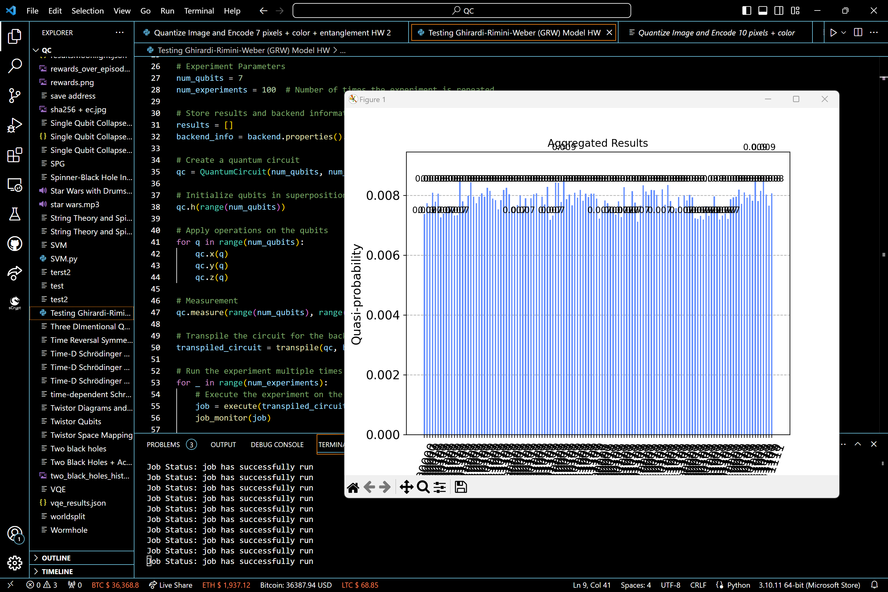
The aggregated results are visualized using a histogram, showing the frequency of each measurement outcome. All results, including the raw data and statistical analysis, are saved to a JSON file for further study or reference.
7. Result Analysis:
The results are returned and saved to a json for further analysis.
Chi-Squared Test:

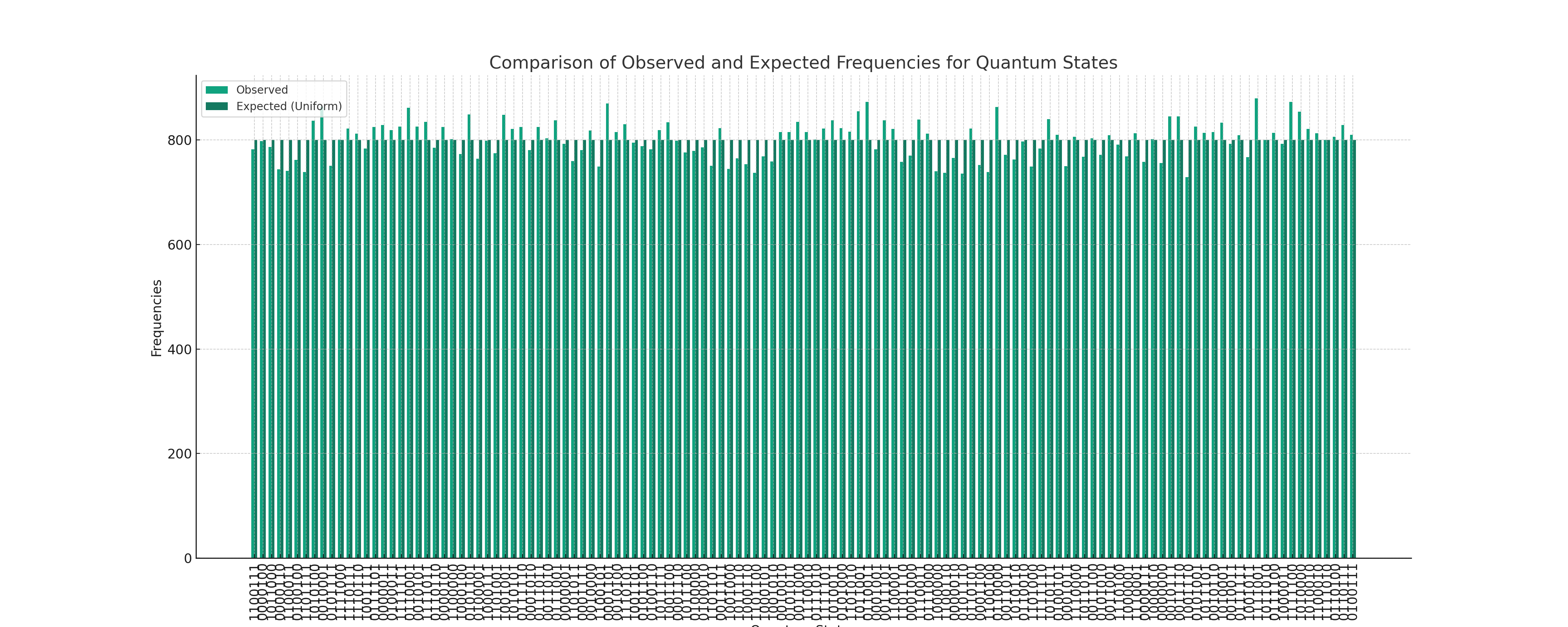
The bar graph above shows comparison between observed and expected frequencies for the quantum states. Each pair of bars represents a quantum state, with the first bar showing the observed frequency and the second bar representing the expected frequency under a uniform distribution. This comparison helps in visually assessing the degree to which the observed data matches or deviates from the expected uniform distribution. Amazingly close!
Mean and Standard Deviation:
Mean Count: Approximately 800. This value represents the average count per quantum state across all experiments.Standard Deviation: Approximately 35.24. This indicates the variability in the counts for different quantum states.
Chi-Squared Test:
Chi-Squared Value: 99.49. This value measures the discrepancy between the observed frequencies and those expected under a uniform distribution.
P-Value:
Approximately 0.966. This high p-value suggests that there is no significant difference between the observed and expected frequencies, implying that the quantum states are uniformly distributed.

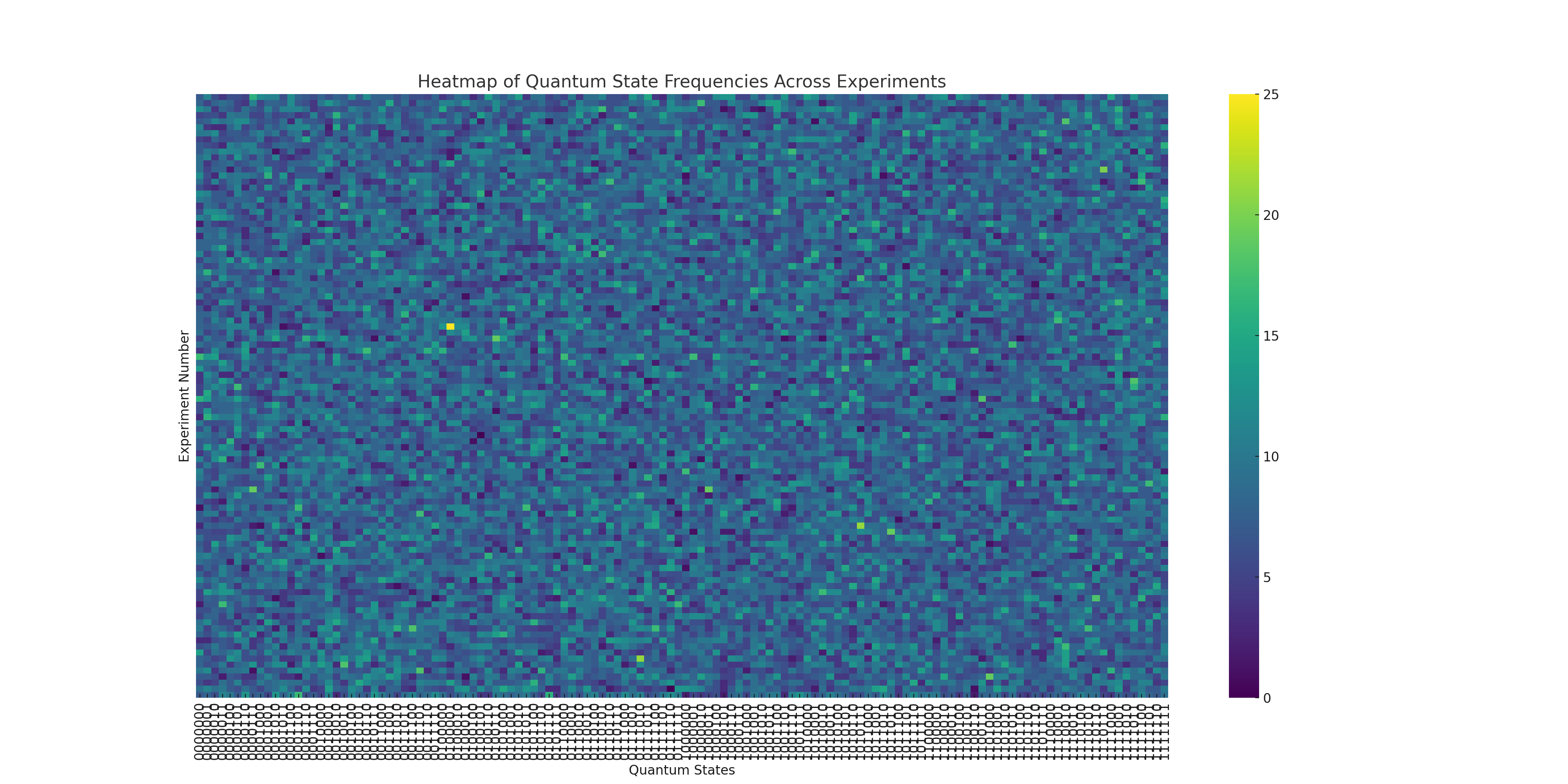
Above is the heatmap of the quantum state frequencies across the experiment. This visualization provides a detailed view of how frequently each quantum state occurred in each experiment. In the heatmap, each row corresponds to one of our experiments, and each column represents a unique quantum state. The color intensity indicates the frequency of each state in each experiment.

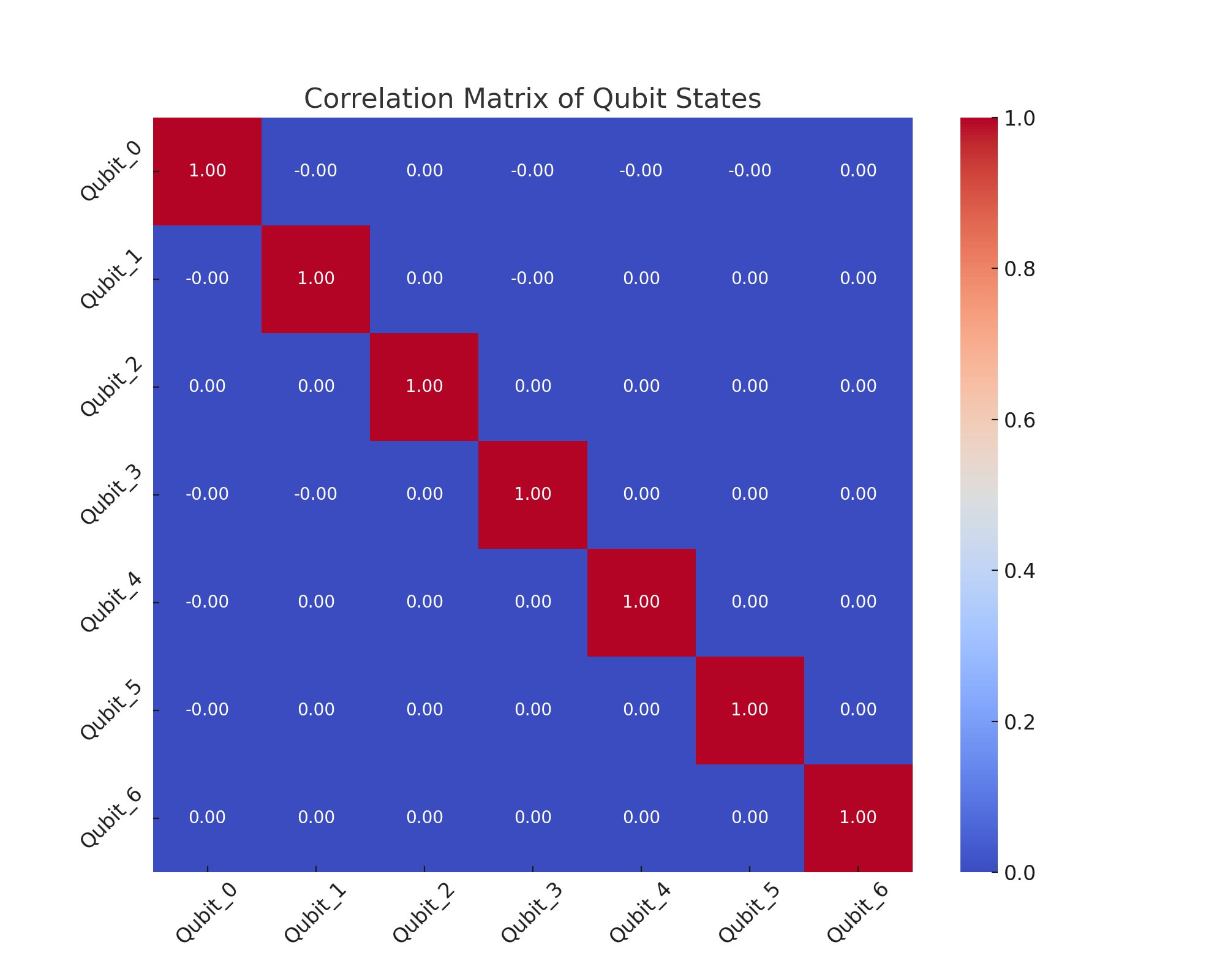
The chart above shows the Correlation Matrix for the states of different qubits. This matrix shows the correlations between the states of different qubits, which can be indicative of entanglement-induced correlations or other quantum interactions.
Each cell in the matrix represents the correlation coefficient between two qubits, with values ranging from -1 (perfect negative correlation) to +1 (perfect positive correlation). A value of 0 indicates no correlation.
In the end, we performed multiple runs to observe the behavior of a 7-qubit system through a series of X, Y, and Z gate operations, followed by measurement. The analysis revealed a uniform distribution of quantum states, as indicated by a high p-value in the chi-squared test, suggesting that the system explored quantum states evenly without bias. The results matched the expected outcome of a uniformly distributed exploration of quantum states, showcasing the potential of quantum systems in exploring complex state spaces.
Code:
import json
from datetime import datetime
from qiskit import QuantumCircuit, transpile, execute
from qiskit.visualization import plot_histogram
from qiskit. tools.monitor import job_monitor
from qiskit_ibm_provider import IBMProvider
import matplotlib.pyplot as plt
import numpy as np
from scipy.stats import chi2_contingency

# Custom JSON Encoder for datetime objects
class CustomEncoder(json.JSONEncoder):
def default(self, obj):
if isinstance(obj, datetime):
return obj.isoformat()
return json.JSONEncoder.default(self, obj)

# Authenticate and load your IBM Q account
IBMProvider. save_account(token='YOUR_TOKEN', overwrite=True)
provider = IBMProvider()

# Access the backend
backend = provider.get_backend('ibm_lagos')
print("Using backend: ", backend)

# Experiment Parameters
num_qubits = 7
num_experiments = 100 # Number of times the experiment is repeated

# Store results and backend information
results = []
backend_info = backend. properties().to_dict()

# Create a quantum circuit
qc = QuantumCircuit(num_qubits, num_qubits)

# Initialize qubits in superposition
qc.h(range(num_qubits))

# Apply operations on the qubits
for q in range(num_qubits):
qc.x(q)
qc.y(q)
qc.z(q)

# Measurement
qc.measure(range(num_qubits), range(num_qubits))

# Transpile the circuit for the backend
transpiled_circuit = transpile(qc, backend)

# Run the experiment multiple times
for _ in range(num_experiments):
# Execute the experiment on the quantum computer
job = execute(transpiled_circuit, backend, shots=1024)
job_monitor(job)

# Collect results
result = job.result()
counts = result.get_counts(qc)
results.append(counts)

# Statistical Analysis
def perform_statistical_analysis(results):
analysis_results = {}
# Aggregate results for each outcome
aggregated_counts = {}
for experiment in results:
for outcome, count in experiment.items():
if outcome not in aggregated_counts:
aggregated_counts[outcome] = 0
aggregated_counts[outcome] += count

# Expected counts for a uniform distribution (no collapse)
expected_counts = [sum(aggregated_counts.values()) / len(aggregated_counts)] * len(aggregated_counts)

# Chi-squared test
chi2, p_value = chi2_contingency([list(aggregated_counts.values()), expected_counts])[:2]
analysis_results = {'chi2': chi2, 'p_value': p_value}
return analysis_results

analysis_results = perform_statistical_analysis(results)

# Plotting and Saving Results
fig, ax = plt.subplots(figsize=(10, 6))

# Aggregate results for plotting
aggregated_counts = {}
for experiment in results:
for outcome, count in experiment.items():
if outcome not in aggregated_counts:
aggregated_counts[outcome] = 0
aggregated_counts[outcome] += count

# Normalize counts
total_counts = sum(aggregated_counts.values())
normalized_counts = {outcome: count / total_counts for outcome, count in aggregated_counts.items()}

# Plot histogram
plot_histogram(normalized_counts, ax=ax)
ax.set_title('Aggregated Results')

plt. show()

# Save results and backend information to a JSON file
experiment_data = {
'results': results,
'analysis': analysis_results,
'backend_info': backend_info
}

with open('experiment_data.json', 'w') as file:
json.dump(experiment_data, file, indent=4, cls=CustomEncoder)

print("Experiment completed. Results and analysis saved to 'experiment_data.json'.")
