Tracing Time-Dependent Quantum State Changes with the Objective Collapse Model on IBM's 7-Qubit Quantum Computer Nairobi
This experiment, using Qiskit, probes Objective Collapse Models (OCM) within quantum mechanics. It involves initializing a complex quantum state, allowing it to evolve, and intermittently measuring it across multiple time steps. The aim is to observe the dynamic time-dependent behavior of quantum states, contributing to the understanding of wave function collapse.
Code Walkthrough
1. Quantum State Preparation:
The experiment begins by preparing a highly entangled quantum state across seven qubits. This is represented mathematically in a Hilbert space, H = C^(2^7), where each qubit contributes a two-dimensional complex vector space.
An entangled state is prepared using the Initialize gate, which is designed to transform the initial state ∣0⟩^(⊗ * 7) into a specified complex superposition state ∣ψ⟩. This state is chosen randomly using random_statevector(2**7).data, creating a vector in the 128-dimensional complex space.
2. Quantum Circuit Evolution:
The Hadamard gate is represented by the unitary matrix:
H = 1/sqrt(2) * (1, 1, 1, −1).
When applied to a single qubit, the Hadamard gate creates a superposition of the basis states. Applying H to the state ∣0⟩ (the standard initial state of a qubit) results in:
H∣0⟩ = 1/sqrt(2) * (∣0⟩ + ∣1⟩).
This operation is crucial for creating states that exhibit quantum interference.
Sequential Application of Gates:
Quantum gates in a circuit are applied in sequence. The overall transformation of the quantum state is represented by the product of the individual gate matrices.
For a sequence of gates G_1, G_2, …, G_n applied to a quantum state ∣ψ⟩, the final state ∣ψ′⟩ is given by:
∣ψ′⟩ = G_n * G_(n−1)… G_2 * G_1 * ∣ψ⟩.
Here, the Hadamard gate is applied to all qubits, and this operation is repeated over five distinct time steps.
Circuit Barrier:
The circuit.barrier() function in Qiskit is used to demarcate different sections of a quantum circuit.
It does not affect the quantum state but prevents certain optimizations that might reorder gates across the barrier during transpilation. This ensures that the sequence of gates is executed as defined.
3. Intermittent Measurements:
At each time step, the quantum state is measured, collapsing the superposition to a definite state. Quantum measurement is described mathematically by projection operators {P_m}, where P_m = ∣m⟩⟨m∣ and ∣m⟩ is a basis state. The probability of collapsing to a particular state ∣m⟩ is given by:
P(m) = ⟨ψ∣P_m∣ψ⟩.
The circuit measures all qubits, translating the quantum state into a classical bit string, across five distinct time steps.
4. Quantum Hardware Execution:
The circuit is transpiled for IBM's 7-Qubit Quantum Computer Nairobi, sent, and processed.
5. Data Collection and Analysis:
The quantum computer returns the measurement results, quantified as the counts of each observed state. This data is collected across all time steps and saved to a json for analysis.

Code:
import numpy as np
from qiskit import IBMQ, transpile
from qiskit.providers.ibmq import least_busy
from qiskit import QuantumCircuit, ClassicalRegister, QuantumRegister
from qiskit.extensions import Initialize
from qiskit.quantum_info import random_statevector
import json
import matplotlib.pyplot as plt

# Input your IBM Q Experience API key here
IBM_API_KEY = 'Your_API_Key' # Replace with your IBM API key

# Load IBM Q account
IBMQ. save_account(IBM_API_KEY, overwrite=True)
IBMQ.load_account()

# Function to create and run the quantum circuit on IBM quantum machine
def run_ocm_experiment(backend):
# Initialize qubits
qreg = QuantumRegister(7)
creg = ClassicalRegister(7)
circuit = QuantumCircuit(qreg, creg)

# Prepare a complex entangled state
init_state = random_statevector(2**7).data
init_gate = Initialize(init_state)
circuit.append(init_gate, qreg)

# Allow state to evolve and perform intermittent measurements
temporal_data = {}
for time_step in range(5):  # Assuming 5 time steps as an example
# Apply some gates for time evolution (example)
circuit.h(qreg)
circuit.barrier()

# Measure some or all qubits
circuit.measure(qreg, creg)

# Transpile for the backend
transpiled_circuit = transpile(circuit, backend)

# Run the circuit on the selected backend
job = backend. run(transpiled_circuit)
result = job.result()

# Collect results
counts = result.get_counts(circuit)
temporal_data[f"Time step {time_step}"] = counts

# Final measurement of all qubits
circuit.measure(qreg, creg)

# Transpile for the backend
transpiled_circuit = transpile(circuit, backend)

# Run the final circuit on the selected backend
job = backend. run(transpiled_circuit)
result = job.result()
final_counts = result.get_counts(circuit)

return {
"temporal_data": temporal_data,
"final_counts": final_counts,
}

# Selecting a quantum computer from IBMQ
provider = IBMQ.get_provider(hub='ibm-q')
backend = least_busy(provider.backends(filters=lambda x: x.configuration().n_qubits >= 7 and not x.configuration().simulator and x.status().operational==True))

# Run the experiment on the selected backend
ocm_results = run_ocm_experiment(backend)

# Save the results to a JSON file
json_file_path = "c:\\Users\\Documents\\OCM_results_data.json"
with open(json_file_path, 'w') as file:
json.dump(ocm_results, file)

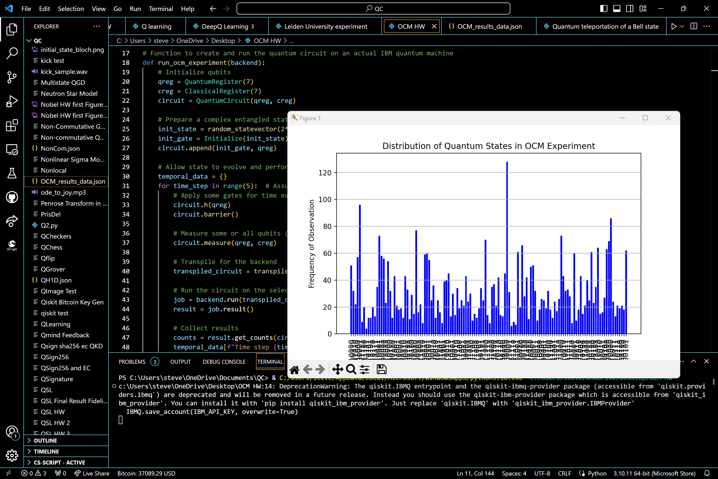
# Displaying a histogram of the final results
states = list(ocm_results['final_counts'].keys())
frequencies = list(ocm_results['final_counts'].values())

plt.figure(figsize=(15, 8))
plt. bar(states, frequencies, color='blue')
plt.xlabel('Quantum States')
plt.ylabel('Frequency of Observation')
plt.title('Distribution of Quantum States in OCM Experiment')
plt.xticks(rotation=90)
plt.grid(axis='y')
plt. show()

print(f"Results saved to {json_file_path}")


Results
Results:
Top 10 states observed:
State: 0000000, Frequency: 128
State: 0000001, Frequency: 96
State: 0010000, Frequency: 86
State: 1000000, Frequency: 77
State: 0010001, Frequency: 73
State: 0001000, Frequency: 73
State: 0011000, Frequency: 70
State: 0000010, Frequency: 69
State: 0000100, Frequency: 66
State: 0010010, Frequency: 64
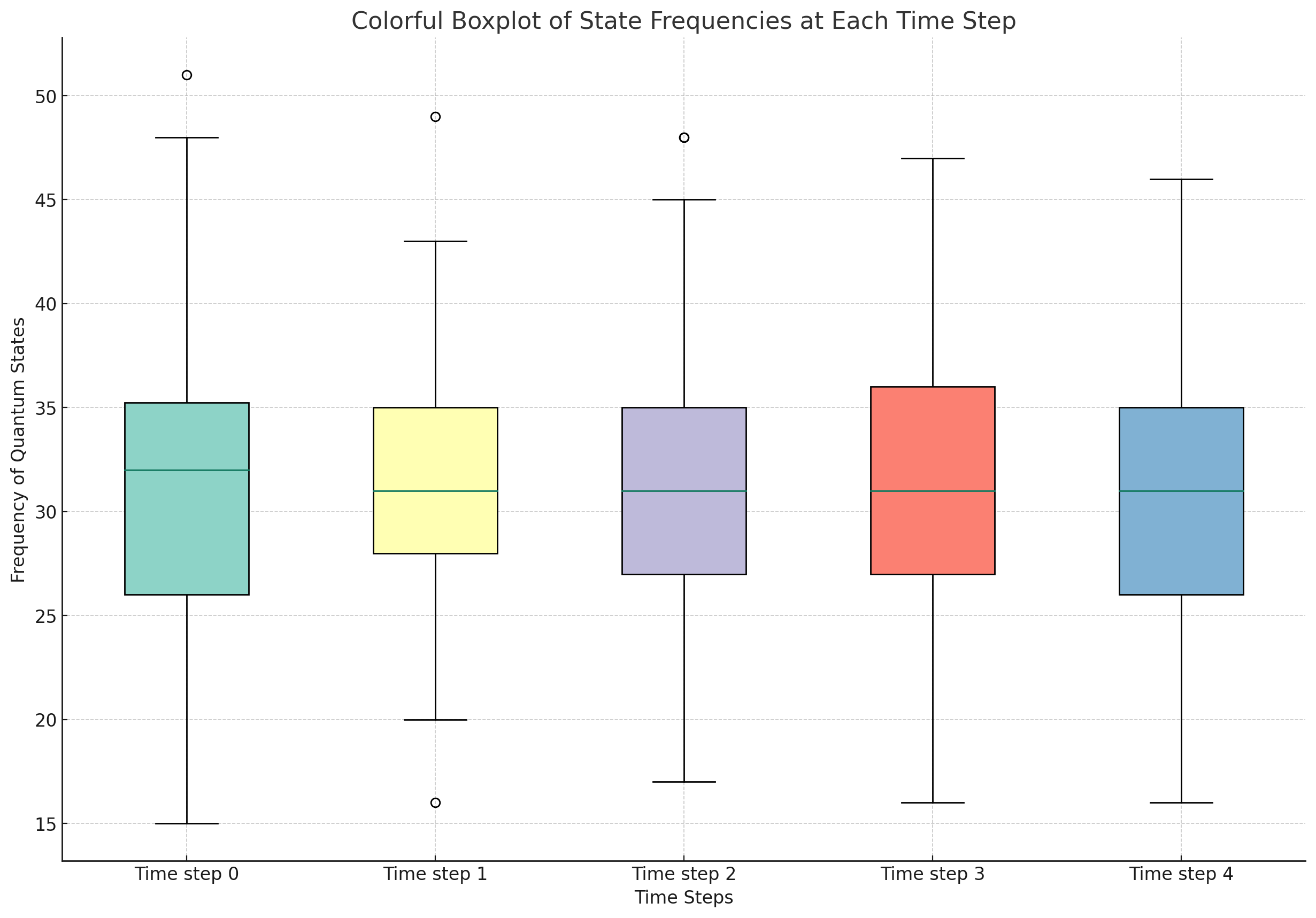
The boxplot above shows the distribution of quantum state frequencies at each time step in the experiment. The length of each box and its whiskers show the range and spread of state frequencies at each time step. A longer box or longer whiskers indicate a greater spread. The line within each box marks the median frequency of states at that time step. Any points outside the whiskers are outliers, representing states with unusually high or low frequencies compared to the majority. Here, we see mostly uniform variance across the time dependent state measurements.
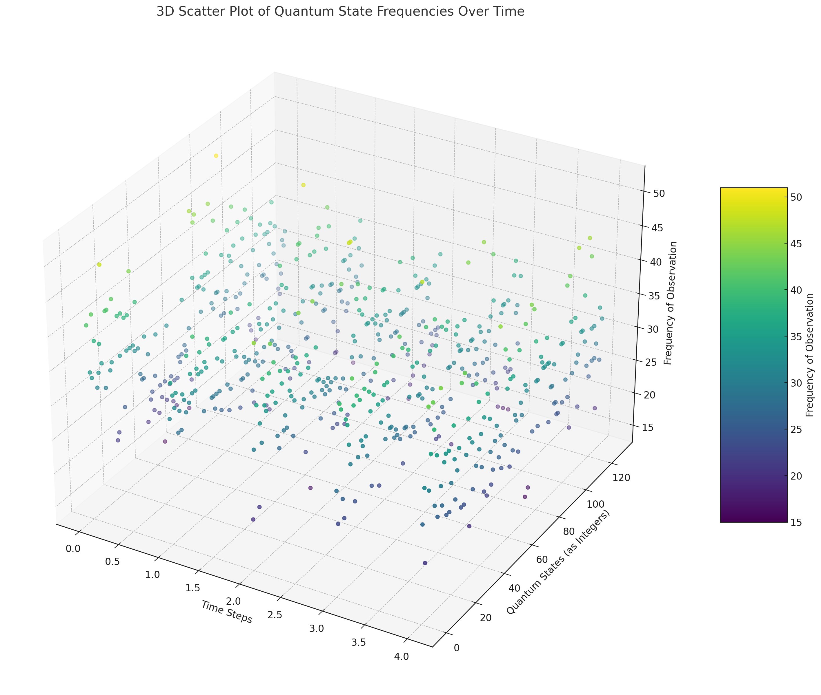
The 3D scatter plot above visualizes the distribution of quantum state frequencies across multiple time steps in the experiment. This plot allows us to observe the spread and dynamics of quantum states in a three-dimensional space. The X-axis represents time steps, the Y-axis shows the quantum states, and the Z-axis indicates the frequency of observation. The color depth (Z-axis) adds an extra dimension of analysis, showing the magnitude of state frequencies. The color and placement of the points illustrate the distribution and density of state observations at each time step. Here, we also see even variability between time dependent state measurements.
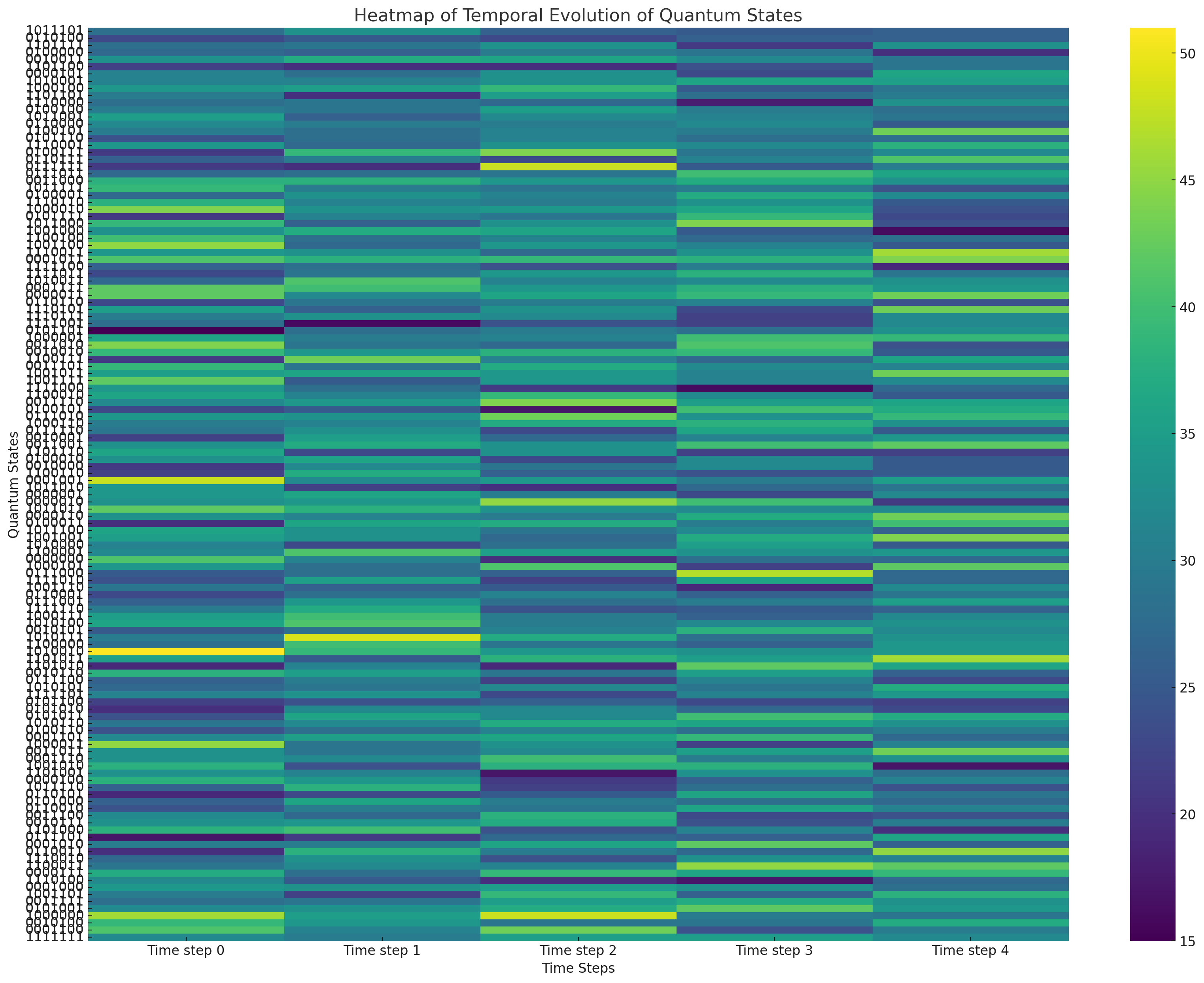
The heatmap above visualizes the temporal evolution of various quantum states in the experiment. Each row represents a different quantum state, and each column corresponds to a time step. The color intensity in each cell indicates the frequency of observation for that state at that time step.
In the end, the data from our experiment revealed significant variability and apparent randomness in the quantum state frequencies. The top states, such as '0000000', '0000001', and '0010000', while more frequent, were part of a broad spectrum of observed states, suggesting a complex and fluctuating quantum landscape. Temporal analysis indicated that the quantum states did not follow a predictable or steady pattern over time. Instead, their frequencies varied significantly at different time steps, illustrating the probabilistic nature of quantum mechanics.
This variability and the absence of a clear, consistent pattern in the temporal evolution of states suggest that quantum state collapse - the transition from a superposition of states to a single state upon observation - is indeed a highly dynamic and non-deterministic process. The experiment underscores the inherent unpredictability and complexity in observing quantum systems, aligning with the fundamental principles of quantum mechanics that emphasize probability and uncertainty.”