Quantum Pixels: Encoding Visual Data within Qubits on IBM's 7-Qubit Quantum Computer Lagos

The experiment, using IBM's 7-qubit quantum computer Lagos and Qiskit, mixes quantum computing with image processing to encode color information into quantum states. By using a series of quantum gates to represent RGB values, the process showcases how quantum mechanics can potentially enhance or provide alternative methods for visual data encoding and retrieval. The end goal is to reconstruct an image's average colors from the quantum-encoded data, assessing the fidelity and exploring the effects of quantum noise and decoherence.

Code Walkthrough

Image Preparation:
A digital image is uploaded. This image is broken up into a matrix I of pixels, where each pixel p_(ij)​ has RGB components (R_(ij) ​,G_(ij)​, B_(ij)​).

Color Data Extraction:
The image I is resized for simplicity, maintaining aspect ratio when necessary, to reduce computational requirements and to adhere to our 7-qubit limit.
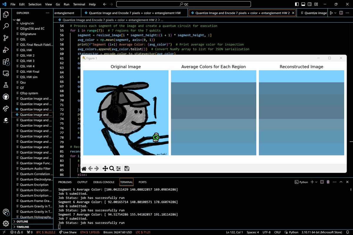
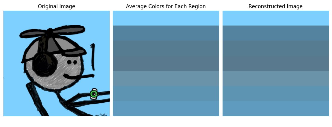
The image is then divided into seven horizontal segments, and for each segment S_k​, the average color C_k ​= (R_k​, G_k​, B_k​) is calculated by averaging the RGB values of all pixels within that segment.

Quantum State Preparation:
The average RGB values are normalized to a [0, 1] range via C_(norm) ​= Ck​/255.
For each color component, a quantum state vector is prepared using rotation gates:
Red intensity is encoded using R_x​(θ_r​) where θ_r​ = 2π⋅R_(norm)​.
Green intensity is encoded using R_y​(θ_g​) where θ_g​ = 2π⋅G_(norm).
Blue intensity is encoded using R_z​(θ_b​) where θ_b ​= 2π⋅B_(norm)​.
The quantum state vector ∣ψ⟩ for each segment is the result of these rotations applied to the initial state ∣000⟩.

Quantum Circuit Execution:
A dynamical decoupling sequence is introduced to counteract decoherence. This is a series of X gates applied at specific intervals, effectively flipping the qubits and refocusing their phase evolution.
The state ∣ψ⟩ is then measured. If the measurement projective operator is M, the measurement result m_k​ for segment k is m_k ​= ⟨ψk​∣M∣ψk​⟩.

Measurement and Error Mitigation:
Calibration circuits are used to characterize the quantum computer's error profile. The Complete Measurement Fitter technique is applied to create a filter that mitigates these errors post-measurement.

Image Reconstruction:
The reconstructed image I is formed by assigning to each segment S_k a color based on the measurement outcome m_k​.
If m_k​ corresponds to 111, the segment is colored with C_k​; otherwise, it is set to black.

Result Visualization and Analysis:
The original, average color, and reconstructed images are visualized to assess the quality of reconstruction and the effects of quantum errors.

Data Saving:
The averaged color values and the quantum measurement results are serialized into a JSON format for documentation and further analysis.

Code:

import cv2
import numpy as np
import matplotlib.pyplot as plt
from qiskit import QuantumCircuit, Aer, execute, IBMQ
from qiskit.visualization import plot_histogram
from qiskit.quantum_info import Statevector
from qiskit.providers.ibmq import least_busy
from qiskit. tools.monitor import job_monitor
from qiskit.ignis.mitigation.measurement import (complete_meas_cal, CompleteMeasFitter)
import json

# Function to encode color information into a quantum state vector using a combination of rotations
def encode_color_to_statevector(color):
    # Normalize the color intensity to be between 0 and 1
    normalized_color = color / 255.0
    # Create a quantum circuit with one qubit for each color channel
    qc = QuantumCircuit(3)
    # Use a combination of X, Y, and Z rotations to encode the color's intensity
    qc.rx(2 * np.pi * normalized_color[0], 0)  # Encoding red intensity
    qc.ry(2 * np.pi * normalized_color[1], 1)  # Encoding green intensity
    qc.rz(2 * np.pi * normalized_color[2], 2)  # Encoding blue intensity
    # Convert the quantum circuit into a state vector
    statevector = Statevector.from_instruction(qc)
    return statevector

# Authenticate and load your IBM Q account
IBMQ. save_account('YOUR_ACCOUNT_NUMBER', overwrite=True)  # Replace 'YOUR_ACCOUNT_NUMBER' with your actual token
IBMQ.load_account()
provider = IBMQ.get_provider(hub='ibm-q')
backend = provider.get_backend('ibm_lagos')
print("Using backend: ", backend)

# Load the original color image
image_path = "C:\\Users\\your image.jpg"  # Replace with your image path
original_image = cv2.imread(image_path)
original_image_rgb = cv2.cvtColor(original_image, cv2.COLOR_BGR2RGB)

# Resize the image to a manageable size for visualization and processing
resized_image = cv2.resize(original_image_rgb, (350, 350), interpolation=cv2.INTER_AREA)

# Divide the resized image into seven equal regions and calculate the average color for each
height, width, _ = resized_image.shape
segment_height = height // 7
avg_colors = []
measurement_results = []

# Measurement calibration circuits (for error mitigation)
cal_circuits, state_labels = complete_meas_cal(qr=QuantumCircuit(3).qregs[0], circlabel='measerrormitigationcal')
cal_jobs = execute(cal_circuits, backend=backend, shots=2000)
job_monitor(cal_jobs)
cal_results = cal_jobs.result()
meas_fitter = CompleteMeasFitter(cal_results, state_labels)

# Process each segment of the image and create a quantum circuit for execution
for i in range(7):  # 7 regions for the 7 qubits
    segment = resized_image[i * segment_height:(i + 1) * segment_height, :]
    avg_color = np.mean(segment, axis=(0, 1))
    print(f"Segment {i+1} Average Color: {avg_color}")  # Print average color for inspection
    avg_colors.append(avg_color.tolist())  # Convert NumPy array to list for JSON serialization
    statevector = encode_color_to_statevector(avg_color)
    # Create a new quantum circuit for state initialization
    qc = QuantumCircuit(3)
    qc.initialize(statevector. data, [0, 1, 2])  # Initialize the qubits with the state vector
    
    # Dynamical decoupling sequence
    qc.barrier()
    qc.x([0, 1, 2])
    qc.barrier()

    qc.measure_all()

    job = execute(qc, backend=backend, shots=2000)
    print(f"Job {i+1} submitted.")
    job_monitor(job)
    result = job.result()
    counts = result.get_counts(qc)
    # Use the maximum occurring result as the measurement result for the segment
    measurement_results.append(1 if counts.get('111', 0) > counts.get('000', 0) else 0)

# Reconstruct the image based on the measurement results
reconstructed_image = np.zeros((segment_height * 7, width, 3), dtype=np.uint8)
for i, measured in enumerate(measurement_results):
    # If measurement is '1', display the color
    if measured:
        reconstructed_image[i * segment_height:(i + 1) * segment_height, :] = np.array(avg_colors[i], dtype=np.uint8)
    else:
        print(f"Segment {i+1} is set to black due to measurement result 0.")

# Assuming you have a list `avg_colors` that stores the average color for each region
# We will create an image to display these average colors
average_colors_image = np.zeros((segment_height * 7, width, 3), dtype=np.uint8)
for i, color in enumerate(avg_colors):
    average_colors_image[i * segment_height:(i + 1) * segment_height, :] = np.array(color, dtype=np.uint8)

# Plot the original image, the average colors image, and the reconstructed image
fig, axs = plt.subplots(1, 3, figsize=(15, 5))  # Create 1 row, 3 columns for subplots

# Display the original image
axs[0].imshow(resized_image)
axs[0].set_title('Original Image')
axs[0].axis('off')

# Display the average colors image
axs[1].imshow(average_colors_image)
axs[1].set_title('Average Colors for Each Region')
axs[1].axis('off')

# Display the reconstructed image
axs[2].imshow(reconstructed_image)
axs[2].set_title('Reconstructed Image')
axs[2].axis('off')

plt.tight_layout()
plt. show()

# Save the results to a JSON file
data_to_save = {
    'average_colors': avg_colors,
    'measurement_results': measurement_results
}
json_path = "C:\\Users\\Desktop\\quantum_image_processing_results.json"
with open(json_path, 'w') as json_file:
    json.dump(data_to_save, json_file, indent=4)
print(f"Results saved to {json_path}")

Results

Using backend: ibm_lagos

Segment 1 Average Color: [125.62651429 207.35737143 254.20622857]

Segment 2 Average Color: [ 83.44891429 131.76605714 159.77874286]

Segment 3 Average Color: [ 86.35022857 124.38394286 146.1144]

Segment 4 Average Color: [ 89.07702857 122.85588571 142.30617143]

Segment 5 Average Color: [106.06211429 146.08822857 169.09834286]

Segment 6 Average Color: [ 92.00165714 148.80108571 178.66074286]

Segment 7 Average Color: [ 94.51754286 155.94182857 191.18114286]

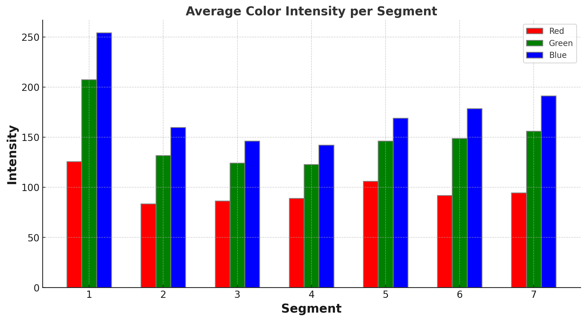
The bar chart above shows the average color intensities for the red, green, and blue channels across each of the seven segments. This visualization allows for an easy comparison of how the color intensities vary between the segments, giving a clear picture of the color distribution throughout the image.

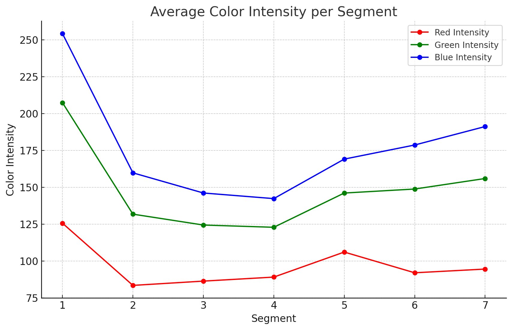
The chart above displays the average color intensities for the red, green, and blue channels across the seven segments of the image. Some observations:
Intensity Variation:
There is a clear variation in intensity levels across the segments, which reflects the different average colors in various parts of the image.
Red Channel:
The red intensity is lowest in the first segment and shows some fluctuation across the segments but generally remains the lowest among the three color channels.
Green Channel:
The green intensity starts lower but increases towards the final segment, suggesting a gradient or a dominant presence of green in the lower parts of the image.
Blue Channel:
The blue channel maintains the highest intensity across all segments, which could indicate a predominance of blue or a consistent background in the image.

In the end, the experiment explores the potential of quantum computing for processing complex datasets such as images, and addresses the challenges posed by errors and noise inherent to current quantum systems. Lagos successfully encoded and retained the color information for all segments of the image, and no segments were lost to measurement errors.