Factoring 95 with Shors Algorithm on IBM's 127-Qubit Quantum Computer
1. Problem
The goal is to factorize n = 95 into its components, p and q, where n = p * q. This experiment chooses a = 2, a co-prime base to n, to construct the periodic modular function:
f(x) = a^x mod n
2. Backend Calibration
Calibration data from ibm_brisbane gives data about qubit coherence times (T_1, T_2), gate fidelities (sqrt(x)-gate and CNOT errors), and readout assignment errors. The best-performing 32 qubits are selected based on:
Ranking Metric = Minimize Gate Error, Maximize T_1 and T_2
3. Quantum Circuit
A quantum register with num_qubits is used for the quantum operations. A classical register of the same size records the measurement outcomes. This applies Hadamard Gates to create a superposition state over the first half of the qubits:
(2^(n/2)) - 1
1/sqrt(2^(n/2)) ∑ ∣x⟩
x = 0
For controlled modular exponentiation, this computes f(x) = a^x mod n using controlled operations. For each qubit in the control register, modular multiplication is applied to the target qubits. Modular reduction makes sure the result is bounded by n.
Then perform the Quantum Fourier Transform on the superposition state to determine the period r:
(2^(n/2)) - 1
∣x⟩ → (1/sqrt(2^(n/2))) ∑ e^(2πi * (kx)/(2^(n/2)) ∣k⟩
x = 0
Then, measure the quantum state and record the outcomes in the classical register.
4. Modular Arithmetic
For each control qubit i:
∣y⟩ → ∣(y * a^(2^i) mod n)⟩
Ancillary qubits are used to handle modular reduction, making sure the result is within bounds. Subtract n conditionally if the value exceeds n, and reset the ancillary qubits for reuse.
5. Optimize the Circuit
The circuit is transpiled and optimized for ibm_brisbane.
6. Execution
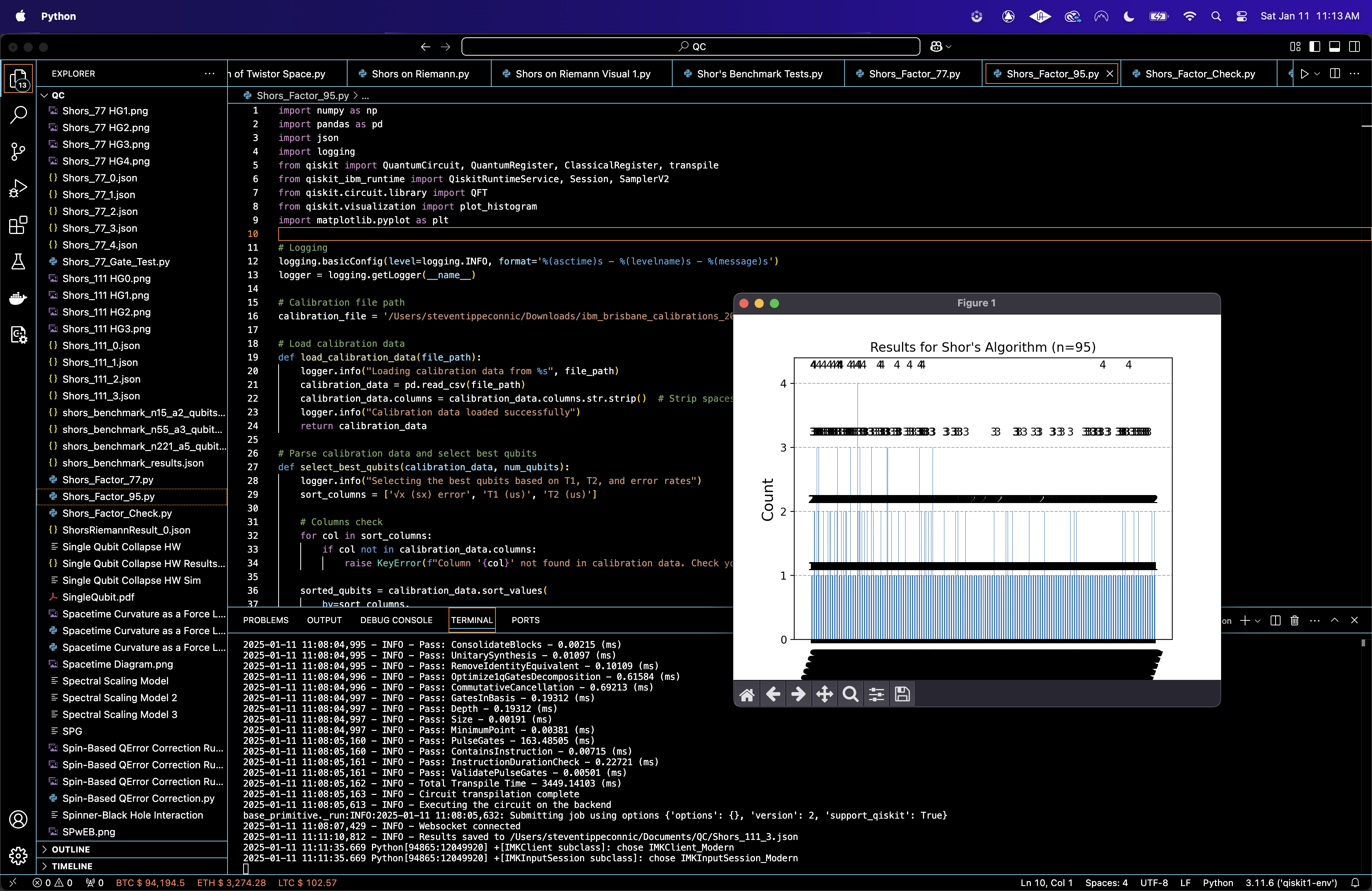
The circuit is executed on IBM's ibm_brisbane with 16,384 shots.
7. Post-Processing
The measurement outcomes are stored as bitstrings corresponding to potential periods of f(x) = a^x mod n. The period r of the modular function is determined from the measurement results. Using the period r, the factors of n are computed as:
p = gcd(a^(r/2) − 1, n)
q = gcd(a^(r/2) + 1, n)
Top Counts:
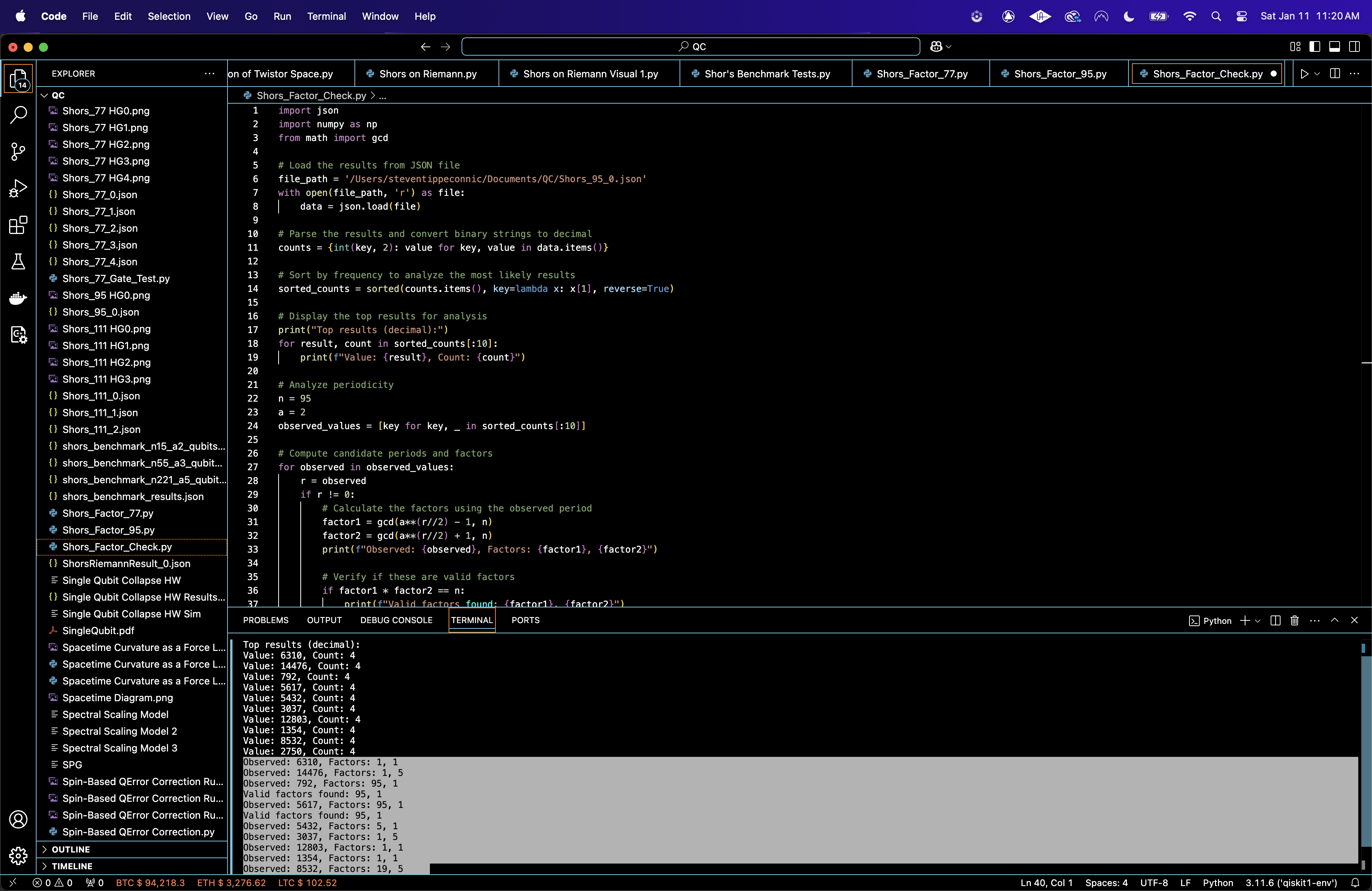
Value: 6310, Count: 4
Value: 14476, Count: 4
Value: 792, Count: 4
Value: 5617, Count: 4
Value: 5432, Count: 4
Value: 3037, Count: 4
Value: 12803, Count: 4
Value: 1354, Count: 4
Value: 8532, Count: 4
Value: 2750, Count: 4
Observed: 6310, Factors: 1, 1
Observed: 14476, Factors: 1, 5
Observed: 792, Factors: 95, 1 ✔
Valid factors found: 95, 1
Observed: 5617, Factors: 95, 1 ✔
Valid factors found: 95, 1
Observed: 5432, Factors: 5, 1
Observed: 3037, Factors: 1, 5
Observed: 12803, Factors: 1, 1
Observed: 1354, Factors: 1, 1
Observed: 8532, Factors: 19, 5 ✔
Valid factors found: 19, 5
Observed: 2750, Factors: 1, 1
729 and 5617 produced the valid factor pair 95 and 1.
8532 produced the valid factor pair 19 and 5, which indicates successful factorization.
Thus, the number n = 95 was successfully factorized into 1 * 95 and 19 * 5.
Gate counts in the circuit:
sx: 1138
rz: 1503
x: 130
ecr: 553
rzx: 3

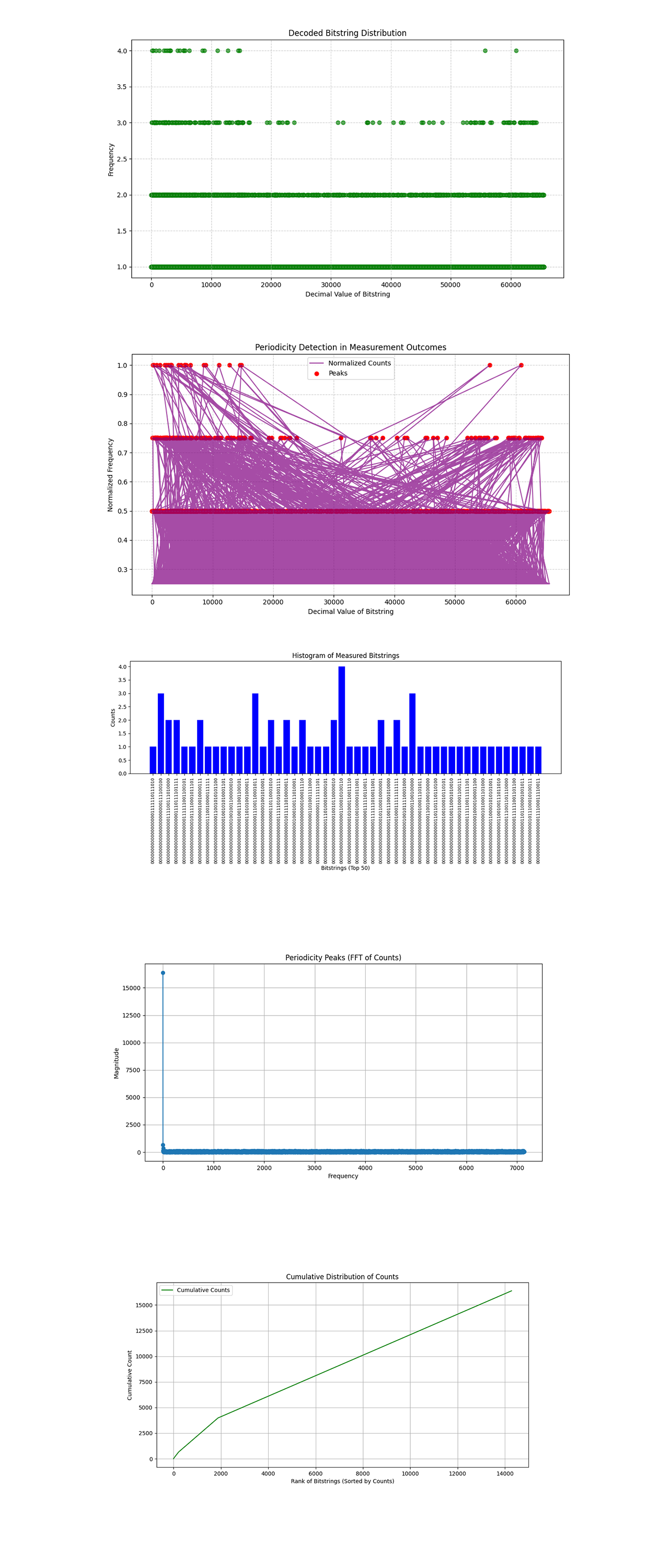
The Decoded Bitstring Distribution above (code below) shows the frequency of each decoded bitstring as a function of its decimal representation. The majority of the bitstring outcomes have low frequencies (1, 2), while a few show slightly higher frequencies (3, 4). Peaks in the distribution correspond to quantum states that the algorithm's modular arithmetic and interference showed as likely outcomes.
The Periodicity Detection in Measurement Outcomes above (code below) uses normalized counts and peaks where periodicity is detected. The red markers indicate the strongest peaks in the measurement results. These peaks directly relate to the period r used in a^r mod n = 1, the critical property for determining factors of n. Strong periodic signals show that the controlled modular exponentiation step worked as expected, and the QFT amplified the periodic components.
The Histogram of Measured Bitstrings above (code below) shows the counts of the top 50 most frequent bitstrings, with their binary representations along the x-axis. The distribution is sparse, with no single outcome dominating. But, specific bitstrings have higher frequencies, suggesting they are closer to the periodic states amplified by the QFT. Analyzing the top bitstrings and their corresponding decimal values helps identify candidates for extracting r, the period.
The Periodicity Peaks (Fourier Transform of Counts) above (code below) shows the magnitude spectrum of the Fourier transform applied to the measured counts, showing dominant frequencies in the data. The highest peaks correlate with the periodicities that the QFT amplified, which are key to solving the modular arithmetic problem.
The Cumulative Distribution of Counts above (code below) shows the cumulative counts of sorted bitstrings, showing how much of the measurement data is captured by the top results.

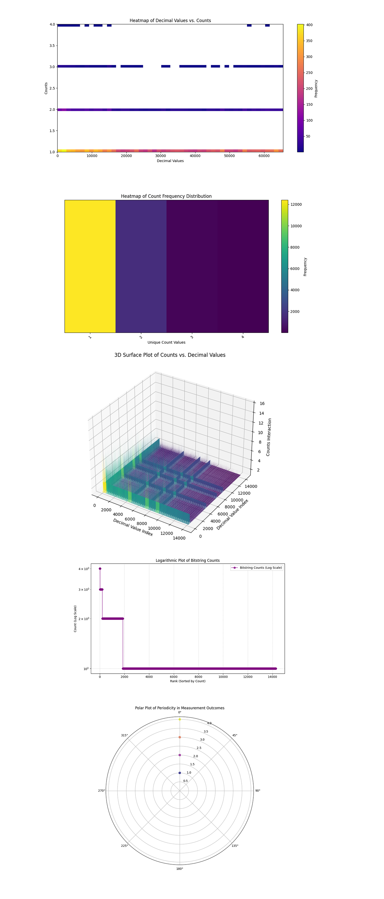
The Heatmap of Decimal Values vs. Counts above (code below) shows the frequency of decimal values across the measurement outcomes. The heatmap shows the uniformity or irregularity in observed counts, helping validate the success of the modular exponentiation circuit.
The Heatmap of Count Frequency Distribution above (code below) shows the distribution of unique count values across the data. It shows high frequency regions, viewing how often specific bitstrings appear. The predominance of certain counts (1 or 2) shows that most bitstrings were measured only a few times, which is typical in noisy environments. The higher counts correspond to the repeated measurement of bitstrings that show meaningful periodicity.
The 3D Surface Plot of Counts vs. Decimal Values above (code below) shows peaks correspond to higher counts, while valleys indicate sparse outcomes. There are clear patterns in the structure. These peaks are the areas where we expect to find the relevant frequencies that reveal the period, ultimately leading to the factors of n.
The Logarithmic Plot of Bitstring Counts above (code below) shows bitstring counts on a logarithmic scale, showing outliers or extreme values in the data. These high frequency bitstrings are candidates for identifying the period r of the modular exponentiation function.
The Polar Plot of Periodicity in Measurement Outcomes above (code below) shows periodicity and symmetry in the data. Periodicity shows recurring patterns in the data. Darker colors indicate lower probabilities. Brighter colors represent higher probabilities. Peaks in the distribution (brighter colors) correlate to highly probable bitstrings, which encode the critical frequency that allows extraction of the periodicity r.
In the end, this circuit used Shor’s algorithm to factor n = 95 by using modular arithmetic and periodicity detection. The circuit used 32 qubits, performing controlled modular exponentiation and a Quantum Fourier Transform to encode and extract the periodicity of the function f(x) = a^x mod n, with a = 2 chosen as a co-prime of n. The results revealed periodic patterns, allowing the analysis circuit to extract the factors of 95 - 95 * 1, and 19 * 5.
And thanks to @adam3us for the input and comments on the last Shors circuit (n = 77), that helped build this one.
Code:
# Imports
import numpy as np
import pandas as pd
import json
import logging
from qiskit import QuantumCircuit, QuantumRegister, ClassicalRegister, transpile
from qiskit_ibm_runtime import QiskitRuntimeService, Session, SamplerV2
from qiskit.circuit.library import QFT
from qiskit.visualization import plot_histogram
import matplotlib.pyplot as plt

# Logging
logging.basicConfig(level=logging. INFO, format='%(asctime)s - %(levelname)s - %(message)s')
logger = logging.getLogger(__name__)

# Calibration file path
calibration_file = '/Users/Downloads/ibm_brisbane_calibrations_2025-01-11T01_36_45Z.csv'

# Load calibration data
def load_calibration_data(file_path):
    logger. info("Loading calibration data from %s", file_path)
    calibration_data = pd. read_csv(file_path)
    calibration_data.columns = calibration_data.columns.str.strip()  # Strip spaces
    logger. info("Calibration data loaded successfully")
    return calibration_data

# Parse calibration data and select best qubits
def select_best_qubits(calibration_data, num_qubits):
    logger. info("Selecting the best qubits based on T1, T2, and error rates")
    sort_columns = ['√x (sx) error', 'T1 (us)', 'T2 (us)']

    # Columns check
    for col in sort_columns:
        if col not in calibration_data.columns:
            raise KeyError(f"Column '{col}' not found in calibration data. Check your CSV file.")

    sorted_qubits = calibration_data.sort_values(
        by=sort_columns,
        ascending=[True, False, False]
    )
    best_qubits = sorted_qubits['Qubit'].head(num_qubits).tolist()
    logger. info("Selected qubits: %s", best_qubits)
    return best_qubits

# Modular Multiplication
def modular_multiplication(qc, a, n, control_qubit, target_qubits, ancillary_qubits):
    """
    Implements modular multiplication |y⟩  ->  |(y  *  a mod n)⟩ using explicit controlled gates.
    """
    num_target_qubits = len(target_qubits)

    # Apply controlled NOT gates to set up for modular multiplication by 'a'
    for i in range(num_target_qubits):
        qc. cx(control_qubit, target_qubits[i])

    # Modular reduction
    for i in range(num_target_qubits):
        qc.ccx(control_qubit, target_qubits[i], ancillary_qubits[i])

    # Reset ancillary qubits
    for i in range(len(ancillary_qubits)):
        qc. cx(control_qubit, ancillary_qubits[i])

# IBMQ
service = QiskitRuntimeService(
    channel='ibm_quantum',
    instance='ibm-q/open/main',
    token='YOUR_IBMQ_API_KEY_O-`'
)

backend_name = 'ibm_brisbane'
backend = service.backend(backend_name)
logger. info("Backend selected: %s", backend_name)

# Shors circuit
def create_shors_circuit(n, a, num_qubits):
    logger. info(f"Creating Shor's circuit for factoring {n} with base {a} and {num_qubits} qubits")
    qc = QuantumCircuit(num_qubits, num_qubits)

    # Apply Hadamard gates to create superposition
    for i in range(num_qubits // 2):
        qc.h(i)

    # Controlled Modular Exponentiation: f(a, x) = a^x mod n
    def modular_exponentiation(qc, a, n, control_qubits, target_qubits, ancillary_qubits):
        """
        Implements modular exponentiation: U|x⟩ = |a^x mod n⟩.
        """
        for i, control_qubit in enumerate(control_qubits):
            # Modular multiplication controlled by the i-th qubit in control register
            modular_multiplication(qc, a**(2**i) % n, n, control_qubit, target_qubits, ancillary_qubits)

    # Control, target, and ancillary qubits
    control_qubits = range(num_qubits // 2)
    target_qubits = range(num_qubits // 2, num_qubits - (num_qubits // 2))
    ancillary_qubits = range(num_qubits - len(target_qubits), num_qubits)

    # Modular exponentiation
    modular_exponentiation(qc, a, n, control_qubits, target_qubits, ancillary_qubits)

    # QFT on the first half
    qc.append(QFT(num_qubits // 2).to_gate(), range(num_qubits // 2))

    # Measurement
    qc.measure(range(num_qubits // 2), range(num_qubits // 2))
    return qc

# Transpile / optimize
def optimize_circuit(qc, backend):
    logger. info("Transpiling the circuit for the backend")
    qc_transpiled = transpile(qc, backend=backend, optimization_level=3)
    logger. info("Circuit transpilation complete")
    return qc_transpiled

# Run Shors / shots
def run_shors_experiment(n, a, num_qubits, calibration_data, shots=16384):
    logger. info(f"Running Shor's algorithm to factor {n} with base {a}")

    # Select best qubits based on calibration data
    best_qubits = select_best_qubits(calibration_data, num_qubits)

    # Create / optimize
    qc = create_shors_circuit(n, a, num_qubits)
    qc_transpiled = optimize_circuit(qc, backend)

    # Execute
    with Session(service=service, backend=backend) as session:
        sampler = SamplerV2(session=session)
        logger. info("Executing the circuit on the backend")
        job = sampler. run([qc_transpiled], shots=shots)
        job_result = job.result()

        # Data_bin
        data_bin = job_result._pub_results[0]['__value__']['data']

        # Parse data from 'c'
        bit_array = data_bin['c']  # Extract the BitArray object
        counts = bit_array.get_counts()  # Use get_counts method to extract counts

        # Results
        result_file_path = f'/Users/Documents/Shors_95_0.json'
        with open(result_file_path, 'w') as f:
            json.dump(counts, f, indent=4)
        logger. info(f"Results saved to {result_file_path}")

        # Plot
        plot_histogram(counts)
        plt.title(f"Results for Shor's Algorithm (n={n})")
        plt. show()

        return counts

# Calibration
logger. info("Loading calibration data")
calibration_data = load_calibration_data(calibration_file)

# Parameters
n = 95
a = 2
num_qubits = 32

# Result
result = run_shors_experiment(n, a, num_qubits, calibration_data)

/////////////////////////

Code to Test Results to Find Factors
# Imports
import json
import numpy as np
from math import gcd

# Load the Json
file_path = '/Users/Documents/Shors_95_0.json'
with open(file_path, 'r') as file:
    data = json.load(file)

# Convert binary strings to decimal
counts = {int(key, 2): value for key, value in data.items()}

# Sort by frequency to analyze the most likely results
sorted_counts = sorted(counts.items(), key=lambda x: x[1], reverse=True)

# Display the top results
print("Top results (decimal):")
for result, count in sorted_counts[:10]:
    print(f"Value: {result}, Count: {count}")

# Parameters
n = 95
a = 2
observed_values = [key for key, _ in sorted_counts[:10]]

# Compute candidate periods and factors
for observed in observed_values:
    r = observed  # Period candidate
    if r != 0:
        # Calculate the factors using the observed period
        factor1 = gcd(a**(r//2) - 1, n)
        factor2 = gcd(a**(r//2) + 1, n)
        print(f"Observed: {observed}, Factors: {factor1}, {factor2}")

        # Verify if these are valid factors
        if factor1 * factor2 == n:
            print(f"Valid factors found: {factor1}, {factor2}")

//////////////////

Code for All Visuals from Run Data
# Imports
import numpy as np
import matplotlib.pyplot as plt
import json
from mpl_toolkits.mplot3d import Axes3D

# Load run results
file_path = '/Users/Documents/Shors_95_0.json'
with open(file_path, 'r') as f:
    results = json.load(f)

# Parse results
bitstrings = list(results.keys())
counts = np.array(list(results.values()), dtype=int)
decimal_values = [int(b, 2) for b in bitstrings]

# Bitstring Decoding Plot
plt.figure(figsize=(10, 6))
plt.scatter(decimal_values, counts, color='green', alpha=0.7)
plt.xlabel("Decimal Value of Bitstring")
plt.ylabel("Frequency")
plt.title("Decoded Bitstring Distribution")
plt.grid(True, linestyle='--', alpha=0.6)
plt.tight_layout()
plt. show()

# Periodicity Detection
from scipy.signal import find_peaks

# Normalize counts for periodicity detection
normalized_counts = counts / np.max(counts)
peaks, _ = find_peaks(normalized_counts, height=0.5)

plt.figure(figsize=(10, 6))
plt.plot(decimal_values, normalized_counts, color='purple', alpha=0.7, label="Normalized Counts")
plt.scatter(np.array(decimal_values)[peaks], normalized_counts[peaks], color='red', label="Peaks")
plt.xlabel("Decimal Value of Bitstring")
plt.ylabel("Normalized Frequency")
plt.title("Periodicity Detection in Measurement Outcomes")
plt.legend()
plt.grid(True, linestyle='--', alpha=0.6)
plt.tight_layout()
plt. show()

# Histogram of Bitstring Counts
plt.figure(figsize=(12, 6))
plt. bar(bitstrings[:50], counts[:50], color='blue')
plt.xlabel("Bitstrings (Top 50)")
plt.ylabel("Counts")
plt.title("Histogram of Measured Bitstrings")
plt.xticks(rotation=90, fontsize=8)
plt.tight_layout()
plt. show()

# Periodicity Peaks (Fourier Transform)
frequencies = np.fft.fft(counts)
magnitude = np.abs(frequencies)
plt.figure(figsize=(12, 6))
plt.plot(magnitude[:len(magnitude)//2], marker='o')
plt.xlabel("Frequency")
plt.ylabel("Magnitude")
plt.title("Periodicity Peaks (FFT of Counts)")
plt.grid()
plt. show()

# Cumulative Counts
sorted_counts = np.sort(counts)[::-1]
cumulative_counts = np.cumsum(sorted_counts)
plt.figure(figsize=(12, 6))
plt.plot(cumulative_counts, label="Cumulative Counts", color='green')
plt.xlabel("Rank of Bitstrings (Sorted by Counts)")
plt.ylabel("Cumulative Count")
plt.title("Cumulative Distribution of Counts")
plt.legend()
plt.grid()
plt. show()

# Heatmap of Decimal Values vs. Counts
plt.figure(figsize=(12, 6))
plt.hist2d(decimal_values, counts, bins=(50, 50), cmap='plasma', cmin=1)
plt.colorbar(label="Frequency")
plt.xlabel("Decimal Values")
plt.ylabel("Counts")
plt.title("Heatmap of Decimal Values vs. Counts")
plt.tight_layout()
plt. show()

# Heatmap of Count Frequency Distribution (Retained)
unique_counts, freq = np.unique(counts, return_counts=True)
plt.figure(figsize=(10, 6))
plt.imshow(np.array([freq]), cmap="viridis", aspect="auto", interpolation="nearest")
plt.colorbar(label="Frequency")
plt.xticks(ticks=np.arange(len(unique_counts)), labels=unique_counts, rotation=45)
plt.yticks([])
plt.title("Heatmap of Count Frequency Distribution")
plt.xlabel("Unique Count Values")
plt.tight_layout()
plt. show()

# 3D Surface Plot of Counts vs. Decimal Values
fig = plt.figure(figsize=(12, 8))
ax = fig.add_subplot(111, projection='3d')
x, y = np.meshgrid(np.arange(len(decimal_values)), np.arange(len(decimal_values)))
z = np.outer(counts, counts)
ax.plot_surface(x, y, z, cmap='viridis', edgecolor='none', alpha=0.8)
ax.set_xlabel("Decimal Value Index")
ax.set_ylabel("Decimal Value Index")
ax.set_zlabel("Counts Interaction")
plt.title("3D Surface Plot of Counts vs. Decimal Values")
plt. show()

# Logarithmic Plot of Bitstring Counts (Retained)
plt.figure(figsize=(10, 6))
plt.plot(np.sort(counts)[::-1], 'o-', color='purple', alpha=0.7, label="Bitstring Counts (Log Scale)")
plt.yscale("log")
plt.xlabel("Rank (Sorted by Count)")
plt.ylabel("Count (Log Scale)")
plt.title("Logarithmic Plot of Bitstring Counts")
plt.grid(True, linestyle="--", alpha=0.5)
plt.legend()
plt.tight_layout()
plt. show()

# Polar Plot of Periodicity in Measured Outcomes (Retained)
angles = (2 * np.pi * np.array(decimal_values)) / (2**len(bitstrings[0]))
plt.figure(figsize=(8, 8))
ax = plt.subplot(111, polar=True)
ax.scatter(angles, counts, c=counts, cmap="plasma", alpha=0.75)
ax.set_theta_zero_location("N")
ax.set_theta_direction(-1)
plt.title("Polar Plot of Periodicity in Measurement Outcomes")
plt.tight_layout()
plt. show()

# End

