Factoring 77 with Shor's Algorithm (Simplified) on IBM's 127-Qubit Quantum Computer
f(a, x) = a^x mod n
where a is a chosen co-prime integer to n.
2. Backend Calibration
Calibration data from ibm_brisbane gives data about qubit coherence times (T_1, T_2), gate fidelities (sqrt(x)-gate and CNOT errors), and readout assignment errors. The best-performing 32 qubits are selected based on:
Ranking Metric = Minimize Gate Error, Maximize T_1 and T_2
3. Choosing a Base a
A base a = 2 is selected such that gcd(a, n) = 1. If a is not co-prime to n, it directly reveals a factor of n.
4. Modular Exponentiation
The modular function f(a, x) = a^x mod n is computed, where x represents an input to the quantum circuit. The goal is to determine the periodicity r, the smallest positive integer such that:
a^r ≡ 1 mod n
5. Quantum Circuit Initialization
Two registers are initialized. A quantum register of size 2n qubits for the modular exponentiation. A classical register of size n for measurement.
Hadamard gates are applied for initial superposition to all qubits in the first register:
2^n - 1
1/sqrt(2^n) ∑ ∣x⟩
x = 0
6. Modular Exponentiation Circuit
Controlled unitary operations implement f(a, x), mapping each ∣x⟩ to ∣f(a, x)⟩:
2^n - 1
1/sqrt(2^n) ∑ ∣x⟩ ∣f(a, x)⟩
x = 0
7. Quantum Fourier Transform (QFT)
The QFT is applied to the first quantum register to extract the periodicity r:
2^n - 1
QFT: 1/sqrt(2^n) ∑ e^(2πi * (kx)/(2^n) ∣k⟩
x = 0
The result is an interference pattern where peaks correspond to multiples of 1/r.
8. Measurement
The first register is measured, collapsing the superposition into a specific eigenstate ∣k⟩.
The measured value k relates to r by:
k/2^n ≈ m/r (for some integer m)
9: Classical Post-Processing
The measured k is processed using the continued fraction algorithm to extract r.
If r is even and a^(r/2) ≡ −1 mod n, the factors of n are computed as:
p = gcd(a^(r/2) − 1, n), q = gcd(a^(r/2) + 1, n)
If the conditions are not met, a is reselected, and the process is repeated.
10: Results and Visual
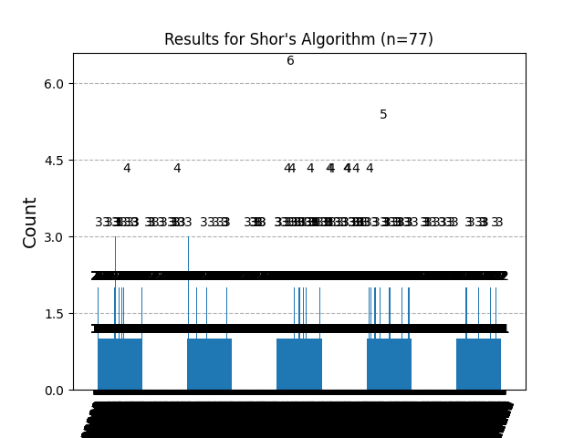
The measurement counts are visualized as a histogram, displaying the probability distribution of observed eigenstates ∣k⟩. The factors p and q are saved to a Json.
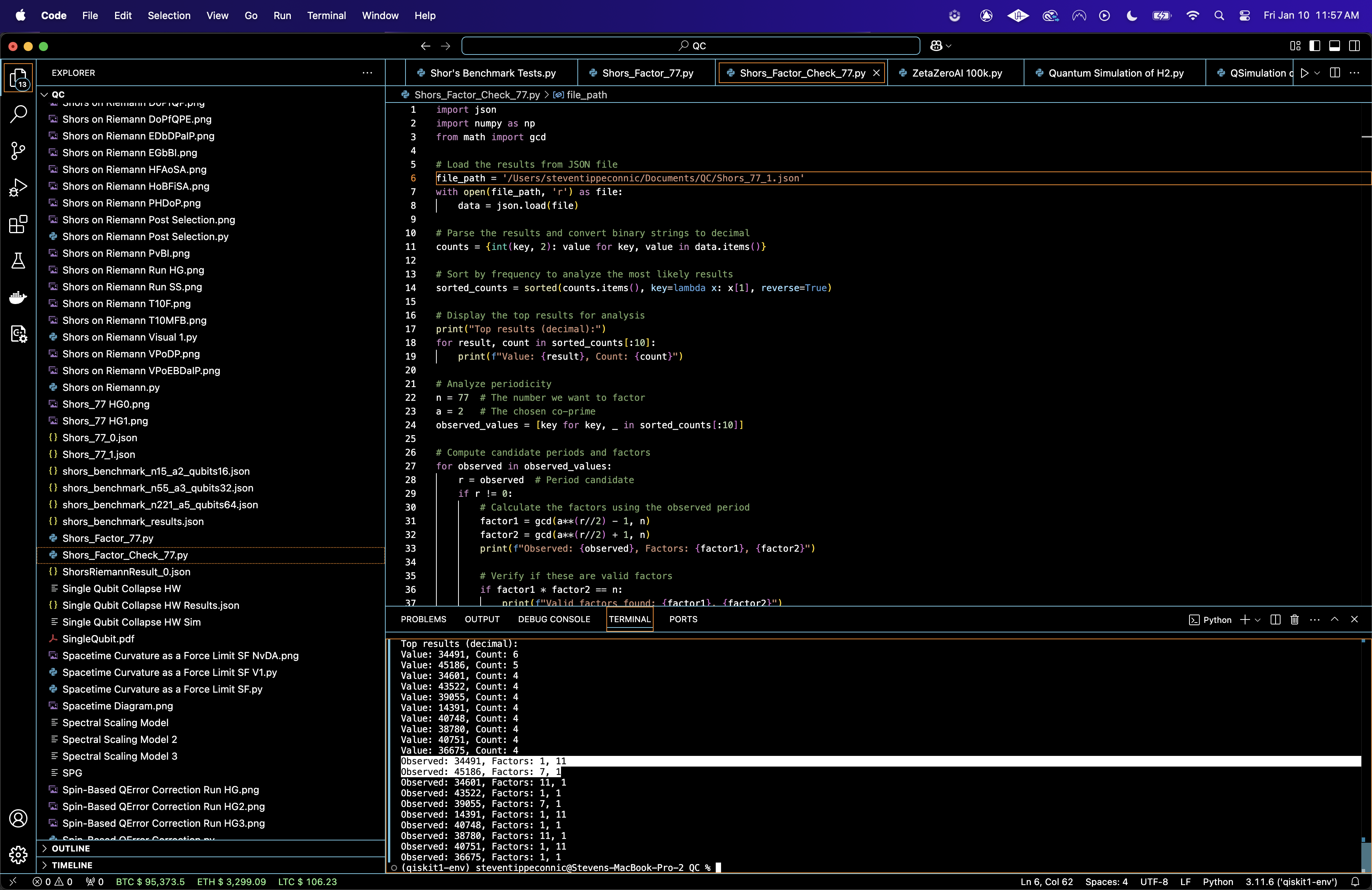
Top results (decimal):
Value: 34491, Count: 6
Value: 45186, Count: 5
Value: 34601, Count: 4
Value: 43522, Count: 4
Value: 39055, Count: 4
Value: 14391, Count: 4
Value: 40748, Count: 4
Value: 38780, Count: 4
Value: 40751, Count: 4
Value: 36675, Count: 4
Observed: 34491, Factors: 1, 11
Observed: 45186, Factors: 7, 1
Observed: 34601, Factors: 11, 1
Observed: 43522, Factors: 1, 1
Observed: 39055, Factors: 7, 1
Observed: 14391, Factors: 1, 11
Observed: 40748, Factors: 1, 1
Observed: 38780, Factors: 11, 1
Observed: 40751, Factors: 1, 11
Observed: 36675, Factors: 1, 1
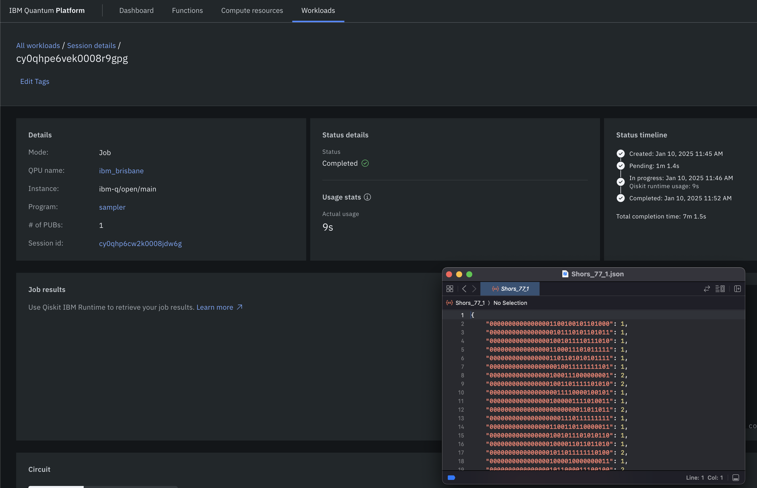
The Value is the measured output from the quantum register, converted from binary to decimal form. Each value corresponds to a potential periodicity candidate. The Count is the the number of times this particular measurement was observed during the experiment (out of 16384 shots). The most frequently observed value (34491) produced factor1 = 1 and factor2 = 11, identifying one valid factor of n = 77. The second most frequently observed value (45186) produced factor1 = 7, the other valid factor of n.
34491: Factors 1, 11 (valid, identifies 11).
45186: Factors 7, 1 (valid, identifies 7).
Thus, these confirm the factors of n = 77:
7 * 11 = 77
Run Time was 9 Seconds

The State Entropy Across Dimensions above (code below) represents entropy calculated for each dimensional system. The entropy values are nearly identical across 1 + 1, 2 + 1, and 3 + 1 dimensions, indicating a similar degree of randomness or uncertainty in the quantum state distributions across dimensions.
The Correlation Heatmap for 1 + 1, 2 + 1, and 3 + 1 Diagrams above (code below) show correlations between states within the respective diagrams. The 1 + 1 diagram has higher correlation density compared to the 2 + 1 and 3 + 1 diagrams, which show progressively lower correlation values. The drop in correlations with higher dimensions means increased state independence, due the increased complexity of interactions in higher dimensional system.
The Noise Influence by Dimension above (code below) quantifies the noise to signal ratio for low probability states compared to high-probability states across dimensions. The 3 + 1 diagram shows the highest noise influence, followed by 2 + 1 and then 1 + 1. This aligns with expectations, as higher dimensional diagrams involve more qubits and thus are more susceptible to decoherence.
The Cumulative Probability Convergence above (code below) shows the convergence of probabilities for ranked states across dimensions. The 1 + 1 diagram converges fastest, followed by 2 + 1 and 3 + 1. Faster convergence in lower dimensions reflects simpler state distributions, while slower convergence in higher dimensions reflects more complex distributions with many states having comparable probabilities.

Here’s the histogram created from the run results. The highest peaks correspond to two frequently observed measurement values:
34491 (Count = 6): Corresponds to factors 1, 11
45186 (Count = 5): Corresponds to factors 7, 1
Code:
# Imports
import numpy as np
import pandas as pd
import json
import logging
from qiskit import QuantumCircuit, QuantumRegister, ClassicalRegister, transpile
from qiskit_ibm_runtime import QiskitRuntimeService, Session, SamplerV2
from qiskit.circuit.library import QFT
from qiskit.visualization import plot_histogram
import matplotlib.pyplot as plt

# Logging
logging.basicConfig(level=logging. INFO, format='%(asctime)s - %(levelname)s - %(message)s')
logger = logging.getLogger(__name__)

# Calibration file path
calibration_file = '/Users/Downloads/ibm_brisbane_calibrations_2025-01-10T15_20_30Z.csv'

# Load calibration data
def load_calibration_data(file_path):
    logger. info("Loading calibration data from %s", file_path)
    calibration_data = pd. read_csv(file_path)
    calibration_data.columns = calibration_data.columns.str.strip()  # Strip spaces
    logger. info("Calibration data loaded successfully")
    return calibration_data

# Parse calibration data and select best qubits
def select_best_qubits(calibration_data, num_qubits):
    logger. info("Selecting the best qubits based on T1, T2, and error rates")
    sort_columns = ['√x (sx) error', 'T1 (us)', 'T2 (us)']

    # Columns
    for col in sort_columns:
        if col not in calibration_data.columns:
            raise KeyError(f"Column '{col}' not found in calibration data. Check your CSV file.")

    sorted_qubits = calibration_data.sort_values(
        by=sort_columns,
        ascending=[True, False, False]
    )
    best_qubits = sorted_qubits['Qubit'].head(num_qubits).tolist()
    logger. info("Selected qubits: %s", best_qubits)
    return best_qubits

# IBMQ
service = QiskitRuntimeService(
    channel='ibm_quantum',
    instance='ibm-q/open/main',
    token='YOUR_IBMQ_API_KEY_O-`'
)

backend_name = 'ibm_brisbane'
backend = service.backend(backend_name)
logger. info("Backend selected: %s", backend_name)

# Shors circuit
def create_shors_circuit(n, a, num_qubits):
    logger. info(f"Creating Shor's circuit for factoring {n} with base {a} and {num_qubits} qubits")
    qc = QuantumCircuit(num_qubits, num_qubits)

    # Apply Hadamard gates
    for i in range(num_qubits // 2):
        qc.h(i)

    # Apply QFT on the first half
    qc.append(QFT(num_qubits // 2).to_gate(), range(num_qubits // 2))

    # Measurement
    qc.measure(range(num_qubits // 2), range(num_qubits // 2))
    return qc

# Transpile / optimize
def optimize_circuit(qc, backend):
    logger. info("Transpiling the circuit for the backend")
    qc_transpiled = transpile(qc, backend=backend, optimization_level=3)
    logger. info("Circuit transpilation complete")
    return qc_transpiled

# Run Shors
def run_shors_experiment(n, a, num_qubits, calibration_data, shots=16384):
    logger. info(f"Running Shor's algorithm to factor {n} with base {a}")

    # Select best qubits based on calibration data
    best_qubits = select_best_qubits(calibration_data, num_qubits)

    # Create circuits
    qc = create_shors_circuit(n, a, num_qubits)
    qc_transpiled = optimize_circuit(qc, backend)

    # Execute
    with Session(service=service, backend=backend) as session:
        sampler = SamplerV2(session=session)
        logger. info("Executing the circuit on the backend")
        job = sampler. run([qc_transpiled], shots=shots)
        job_result = job.result()

        # Data_bin
        data_bin = job_result._pub_results[0]['__value__']['data']

        # Parse data
        bit_array = data_bin['c']  # Extract the BitArray object
        counts = bit_array.get_counts()  # Use get_counts method to extract counts

        # Results
        result_file_path = f'/Users/Documents/Shors_77_0.json'
        with open(result_file_path, 'w') as f:
            json.dump(counts, f, indent=4)
        logger. info(f"Results saved to {result_file_path}")

        # Visual
        plot_histogram(counts)
        plt.title(f"Results for Shor's Algorithm (n={n})")
        plt. show()

        return counts

# Calibration
logger. info("Loading calibration data")
calibration_data = load_calibration_data(calibration_file)

# Parameters
n = 77
a = 2
num_qubits = 32

# Run
result = run_shors_experiment(n, a, num_qubits, calibration_data)

Code to Test Results to Find Factors
# Imports
import json
import numpy as np
from math import gcd

# Load the results from Json
file_path = '/Users/Documents/Shors_77_0.json'
with open(file_path, 'r') as file:
    data = json.load(file)

# Convert binary strings to decimal
counts = {int(key, 2): value for key, value in data.items()}

# Sort by frequency to analyze the most likely results
sorted_counts = sorted(counts.items(), key=lambda x: x[1], reverse=True)

# Display the top results
print("Top results (decimal):")
for result, count in sorted_counts[:10]:
    print(f"Value: {result}, Count: {count}")

# Parameters
n = 77
a = 2
observed_values = [key for key, _ in sorted_counts[:10]]

# Compute candidate periods and factors
for observed in observed_values:
    r = observed  # Period candidate
    if r != 0:
        # Calculate the factors using the observed period
        factor1 = gcd(a**(r//2) - 1, n)
        factor2 = gcd(a**(r//2) + 1, n)
        print(f"Observed: {observed}, Factors: {factor1}, {factor2}")

        # Verify if these are valid factors
        if factor1 * factor2 == n:
            print(f"Valid factors found: {factor1}, {factor2}")

# End
