Exploring State Dynamics in Abstract 1 + 1, 2 + 1, and 3 + 1 Spacetime Dimensions
1. Backend and Calibration
The experiment uses IBM’s ibm_kyiv with 30 qubits. Calibration data is loaded and parsed to select optimal qubits based on error rates (sqrt(x)), T_1, and T_2 coherence times. 10 qubits are allocated for each dimensional simulation (1 + 1, 2 + 1, 3 + 1).
2. 1 + 1 Dimension Construction
A quantum circuit is created with 10 qubits and initialized to ∣0⟩.
Apply a Hadamard gate (H) to the first qubit, creating a superposition:
∣+⟩ = -1/sqrt * (∣0⟩ + ∣1⟩)
Controlled R_x gates (CR_x(θ)) are applied, where the first qubit controls rotations on each subsequent qubit:
θ = π/(2i), i∈{1, 2, …, 9}
R_z(θ) rotations are applied to each subsequent qubit using the same θ.
All 10 qubits are measured.
3. 2 + 1 Dimension Construction
A quantum circuit is created with another set of 10 qubits (qubits 10 - 19) and initialized to ∣0⟩.
Apply H gates to all 10 qubits, creating superpositions.
Controlled R_z gates (CR_z(θ)) are applied between all pairs of qubits:
θ = π/(3(j + 1)), j∈{1, 2, …, 9}
Apply single qubit R_x rotations (π/8) to each qubit to introduce perturbations.
All 10 qubits are measured.
4. 3 + 1 Dimension Construction
A quantum circuit is created with the final set of 10 qubits (qubits 20 - 29) and initialized to ∣0⟩.
Apply H gates to all 10 qubits.
Controlled R_y gates (CR_y(θ)) are applied between all pairs of qubits:
θ = π/(4(j + 1)), j∈{1, 2, …, 9}
Apply single qubit R_z rotations (π/10) to each qubit.
All 10 qubits are measured.
5. Transpile and Execution
Each circuit is transpiled for ibm_kyiv. Each circuit (1 + 1, 2 + 1, 3 + 1) is executed independently with 16,384 shots.
6. Results and Visual
Results are retrieved for each circuit and saved to separate Jsons. The measurement results are visualized as histograms.

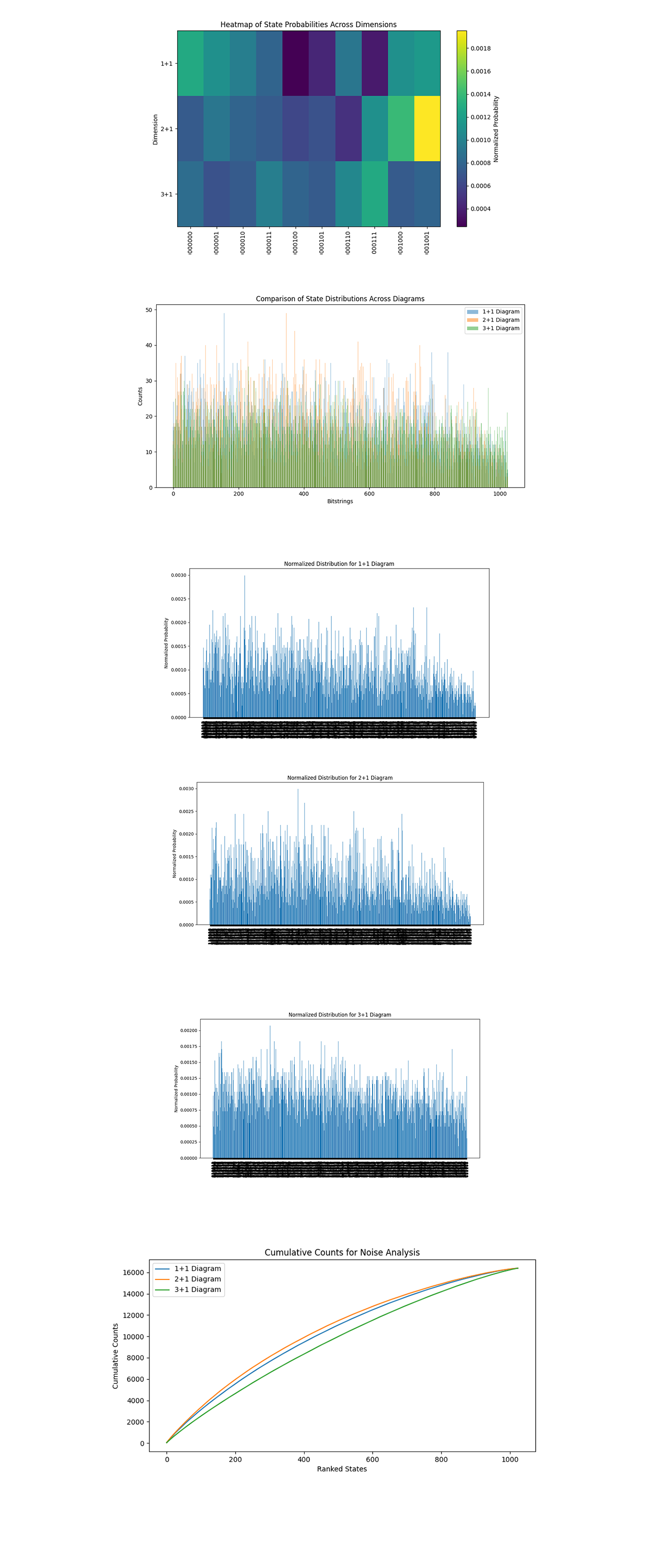
The Heatmap of State Probabilities Across Dimensions above (code below) shows the normalized probabilities of the top 10 bitstring states across the 1 + 1, 2 + 1, and 3 + 1 diagrams. Each row corresponds to a dimension, and each column corresponds to a bitstring state. Bright colors (yellow) indicate higher probabilities, while darker colors (purple/blue) indicate lower probabilities. The 1 + 1 diagram has higher peaks. The 2 + 1 diagram shows a sharp peak in probability for specific states, likely due to stronger correlations or symmetries in the encoding. The 3 + 1 diagram has a more spread out distribution, meaning higher noise or decoherence, as expected with increased qubits.
The Comparison of State Distributions Across Diagrams above (code below) overlays the raw counts of states for each diagram, giving a direct comparison of bitstring distributions. The 1 + 1 diagram has more prominent peaks, meaning fewer states dominating the distribution. This aligns with its simpler coupling structure. The 2 + 1 and 3 + 1 diagrams show a more even spread, meaning increased state mixing due to more complex couplings.
The Normalized Distribution for Each Diagram above (code below) shows the relative frequency of all bitstring states. For 1 + 1, a few states dominate the distribution, with a steep drop off in probabilities for others. This reflects a more structured system. For 2 + 1, the probabilities spread more evenly across states, with multiple high probability peaks. This means stronger entanglement and a more intricate structure. For 3 + 1, the distribution flattens further, with smaller peaks and a broader base.
The Cumulative Counts for Noise Analysis above (code below) shows the sum of state probabilities ranked by frequency for each diagram. Steeper curves indicate fewer high probability states dominating the distribution, while flatter curves indicate more even distributions. The 1 + 1 curve rises steeply initially, showing a few states dominate its distribution. This means a well defined and less noisy simulation. The 2 + 1 curve flattens slightly, indicating a broader distribution of states, likely due to increased entanglement and coupling complexity. The 3 + 1 curve is the flattest, reflecting the most complex system.

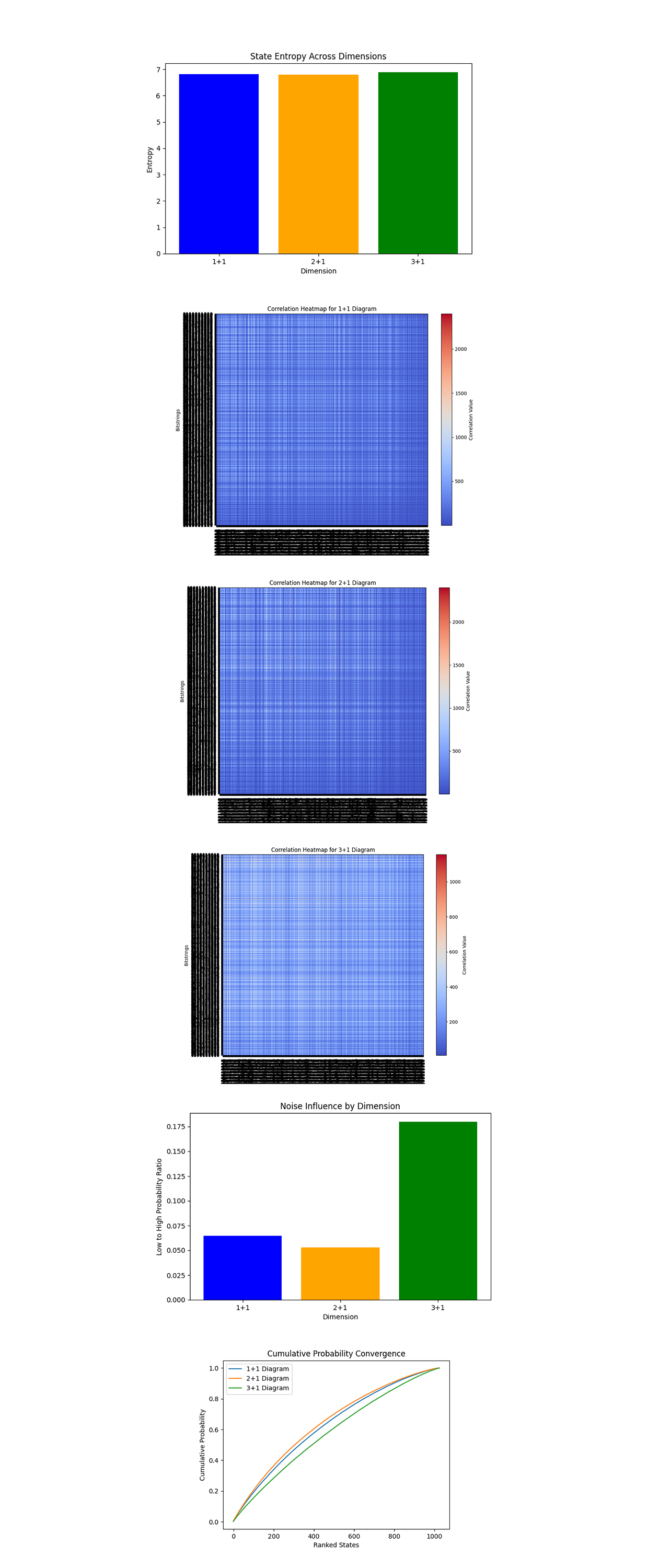
The State Entropy Across Dimensions above (code below) represents entropy calculated for each dimensional system. The entropy values are nearly identical across 1 + 1, 2 + 1, and 3 + 1 dimensions, indicating a similar degree of randomness or uncertainty in the quantum state distributions across dimensions.
The Correlation Heatmap for 1 + 1, 2 + 1, and 3 + 1 Diagrams above (code below) show correlations between states within the respective diagrams. The 1 + 1 diagram has higher correlation density compared to the 2 + 1 and 3 + 1 diagrams, which show progressively lower correlation values. The drop in correlations with higher dimensions means increased state independence, due the increased complexity of interactions in higher dimensional system.
The Noise Influence by Dimension above (code below) quantifies the noise to signal ratio for low probability states compared to high-probability states across dimensions. The 3 + 1 diagram shows the highest noise influence, followed by 2 + 1 and then 1 + 1. This aligns with expectations, as higher dimensional diagrams involve more qubits and thus are more susceptible to decoherence.
The Cumulative Probability Convergence above (code below) shows the convergence of probabilities for ranked states across dimensions. The 1 + 1 diagram converges fastest, followed by 2 + 1 and 3 + 1. Faster convergence in lower dimensions reflects simpler state distributions, while slower convergence in higher dimensions reflects more complex distributions with many states having comparable probabilities.

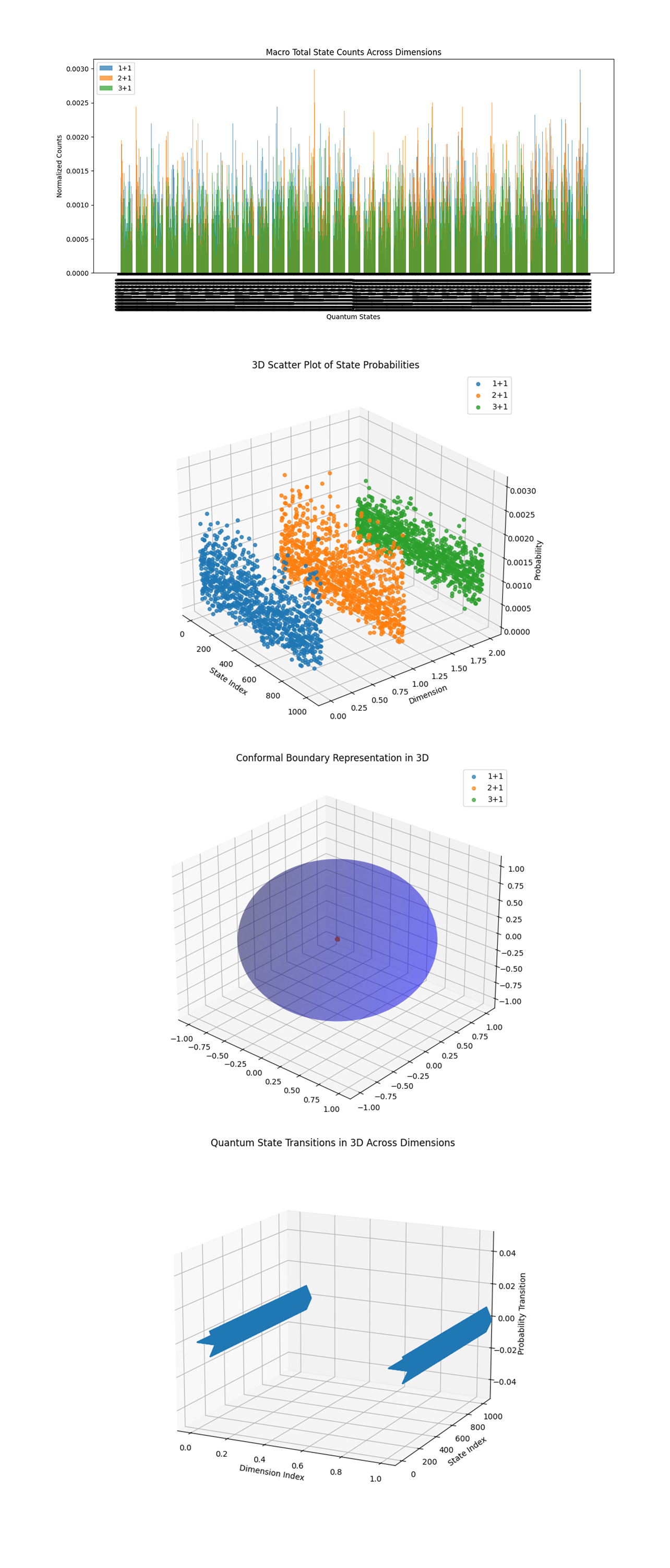
The Macro Total State Counts Across Dimensions above (code below) aggregates normalized counts across all quantum states for the 1 + 1, 2 + 1, and 3 + 1 diagrams. The consistency in the relative distribution among dimensions shows differences in how each configuration explores the state space. The lower overall amplitudes in 3 + 1 mean increased complexity, noise, or diminished state population compared to 1 + 1 and 2 + 1.
The 3D Scatter Plot of State Probabilities above (code below) maps the probabilities for quantum states across dimensions in a 3D space. The clear segmentation of clusters (1 + 1, 2 + 1, 3 + 1) demonstrates distinct probabilistic behaviors in each dimension. The variance within clusters means differing complexity in state distribution, with 3 + 1 exhibiting the widest spread.
The Conformal Boundary Representation in 3D above (code below) abstracts the systems into a conformal boundary representation. The spherical shape aligns with expectations of how light cones and causal structures are represented in conformal geometry. The central red point indicates the convergence of states near a singularity. Higher dimensions (3 + 1) appear to align more tightly to the conformal boundary.
The Quantum State Transitions in 3D Across Dimensions above (code below) shows transitions between high probability states across dimensions. The trajectories mean that quantum evolution in 3 + 1 is more complex and exhibits higher nonlinearity compared to 1 + 1 and 2 + 1.
In the end, this experiment explored quantum systems across different abstract spacetime dimensional constructs - 1 + 1, 2 + 1, and 3 + 1. By constructing quantum circuits to encode the causal structure of these diagrams, this circuit explored probabilistic state distributions, entropy, noise impact, and state transitions as dimensions scaled.
Code:
# Imports
import numpy as np
import pandas as pd
import logging
from qiskit import QuantumCircuit, QuantumRegister, ClassicalRegister, transpile
from qiskit_ibm_runtime import QiskitRuntimeService, Session, SamplerV2
from qiskit.visualization import plot_histogram
import matplotlib.pyplot as plt
import json

# Logging
logging.basicConfig(level=logging. INFO, format='%(asctime)s - %(levelname)s - %(message)s')
logger = logging.getLogger(__name__)

# Load calibration data
def load_calibration_data(file_path):
    logger. info("Loading calibration data from %s", file_path)
    calibration_data = pd. read_csv(file_path)
    calibration_data.columns = calibration_data.columns.str.strip()
    logger. info("Calibration data loaded successfully")
    return calibration_data

# Select optimal qubits based on calibration data
def select_optimal_qubits(calibration_data, num_qubits):
    logger. info("Selecting optimal qubits based on error rates and coherence times")
    qubits_sorted = calibration_data.sort_values(by=['\u221ax (sx) error', 'T1 (us)', 'T2 (us)'], ascending=[True, False, False])
    selected_qubits = qubits_sorted['Qubit'].head(num_qubits).tolist()
    logger. info("Selected qubits: %s", selected_qubits)
    return selected_qubits

# Load calibration data
calibration_file = '/Users/Downloads/ibm_kyiv_calibrations_2025-01-03T00_08_15Z.csv'
calibration_data = load_calibration_data(calibration_file)

# IBMQ
service = QiskitRuntimeService(
    channel='ibm_quantum',
    instance='ibm-q/open/main',
    token='YOUR_IBMQ_API_KEY_O-`'
)
backend_name = 'ibm_kyiv'
backend = service.backend(backend_name)
logger. info("Backend selected: %s", backend_name)

# Qubits
num_qubits = 30
selected_qubits = select_optimal_qubits(calibration_data, num_qubits)

# Quantum and classical registers
qr = QuantumRegister(num_qubits, 'q')
qc_1p1 = QuantumCircuit(qr[:10], name='1+1 Diagram')
qc_2p1 = QuantumCircuit(qr[10:20], name='2+1 Diagram')
qc_3p1 = QuantumCircuit(qr[20:30], name='3+1 Diagram')

# Build 1 + 1 Spacetime diagram
logger. info("Constructing 1+1 Spacetime diagram")
def construct_1p1_diagram(qc, qr):
    for i in range(1, 10):
        qc.h(qr[i])
        coupling_angle = np.pi / (2 * i)
        qc.crx(coupling_angle, qr[0], qr[i])
        qc.rz(coupling_angle, qr[i])

construct_1p1_diagram(qc_1p1, qr[:10])

# Build 2 + 1 Spacetime diagram
logger. info("Constructing 2+1 Spacetime diagram")
def construct_2p1_diagram(qc, qr_subset):
    for i in range(len(qr_subset)):
        qc.h(qr_subset[i])
        for j in range(len(qr_subset)):
            if i != j:  # Avoid duplicate qubits
                coupling_angle = np.pi / (3 * (j + 1))
                qc.crz(coupling_angle, qr_subset[j], qr_subset[i])
        qc.rx(np.pi / 8, qr_subset[i])

construct_2p1_diagram(qc_2p1, qr[10:20])

# Build 3 + 1 Spacetime diagram
logger. info("Constructing 3+1 Spacetime diagram")
def construct_3p1_diagram(qc, qr_subset):
    for i in range(len(qr_subset)):
        qc.h(qr_subset[i])
        for j in range(len(qr_subset)):
            if i != j:  # Avoid duplicate qubits
                coupling_angle = np.pi / (4 * (j + 1))
                qc.cry(coupling_angle, qr_subset[j], qr_subset[i])
        qc.rz(np.pi / 10, qr_subset[i])

construct_3p1_diagram(qc_3p1, qr[20:30])

# Measure 1 + 1
cr_1p1 = ClassicalRegister(10, 'meas_1p1')
qc_1p1.add_register(cr_1p1)
qc_1p1.measure(qr[:10], cr_1p1)

# Measure 2 + 1
cr_2p1 = ClassicalRegister(10, 'meas_2p1')
qc_2p1.add_register(cr_2p1)
qc_2p1.measure(qr[10:20], cr_2p1)

# Measure 3 + 1
cr_3p1 = ClassicalRegister(10, 'meas_3p1')
qc_3p1.add_register(cr_3p1)
qc_3p1.measure(qr[20:30], cr_3p1)

# Transpile
logger. info("Transpiling the quantum circuits for the backend")
qc_1p1_transpiled = transpile(qc_1p1, backend=backend, initial_layout=selected_qubits[:10], optimization_level=3)
qc_2p1_transpiled = transpile(qc_2p1, backend=backend, initial_layout=selected_qubits[10:20], optimization_level=3)
qc_3p1_transpiled = transpile(qc_3p1, backend=backend, initial_layout=selected_qubits[20:30], optimization_level=3)
logger. info("Circuit transpilation complete")

# Execute
shots = 16384
with Session(service=service, backend=backend) as session:
    sampler = SamplerV2(session=session)

    # 1 + 1
    logger. info("Executing the 1+1 diagram circuit on the backend")
    job_1p1 = sampler. run([qc_1p1_transpiled], shots=shots)
    job_result_1p1 = job_1p1.result()
    counts_1p1 = job_result_1p1._pub_results[0]['__value__']['data']['meas_1p1'].get_counts()

    results_data_1p1 = {"raw_counts": counts_1p1}
    file_path_1p1 = '/Users/Documents/QSpacetime_1p1.json'
    with open(file_path_1p1, 'w') as f:
        json.dump(results_data_1p1, f, indent=4)
    logger. info("1+1 results saved to %s", file_path_1p1)

    # 2 + 1
    logger. info("Executing the 2+1 diagram circuit on the backend")
    job_2p1 = sampler. run([qc_2p1_transpiled], shots=shots)
    job_result_2p1 = job_2p1.result()
    counts_2p1 = job_result_2p1._pub_results[0]['__value__']['data']['meas_2p1'].get_counts()

    results_data_2p1 = {"raw_counts": counts_2p1}
    file_path_2p1 = '/Users/Documents/QSpacetime_2p1.json'
    with open(file_path_2p1, 'w') as f:
        json.dump(results_data_2p1, f, indent=4)
    logger. info("2+1 results saved to %s", file_path_2p1)

    # 3+1
    logger. info("Executing the 3+1 diagram circuit on the backend")
    job_3p1 = sampler. run([qc_3p1_transpiled], shots=shots)
    job_result_3p1 = job_3p1.result()
    counts_3p1 = job_result_3p1._pub_results[0]['__value__']['data']['meas_3p1'].get_counts()

    results_data_3p1 = {"raw_counts": counts_3p1}
    file_path_3p1 = '/Users/Documents/QSpacetime_3p1.json'
    with open(file_path_3p1, 'w') as f:
        json.dump(results_data_3p1, f, indent=4)
    logger. info("3+1 results saved to %s", file_path_3p1)

# Visuals
plot_histogram(counts_1p1)
plt.title("1+1 Diagram Quantum Simulation")
plt. show()

plot_histogram(counts_2p1)
plt.title("2+1 Diagram Quantum Simulation")
plt. show()

plot_histogram(counts_3p1)
plt.title("3+1 Diagram Quantum Simulation")
plt. show()

//////////////////////////////////
# Imports
import matplotlib.pyplot as plt
from qiskit.visualization import plot_histogram
import json
from itertools import accumulate
import numpy as np
from scipy.stats import entropy
from mpl_toolkits.mplot3d import Axes3D

# File paths
file_paths = [
    '/Users/Documents/QSpacetime_1p1.json',
    '/Users/Documents/QSpacetime_2p1.json',
    '/Users/Documents/QSpacetime_3p1.json'
]

# Load Raw Counts
results = []
for file_path in file_paths:
    with open(file_path, 'r') as file:
        results.append(json.load(file)["raw_counts"])

# Data Sets
data = []  # Initialize data list
for file_path in file_paths:
    try:
        with open(file_path, 'r') as f:
            content = json.load(f)  # Load JSON content
            if 'raw_counts' in content:
                data.append(content['raw_counts'])
            else:
                print(f"Key 'raw_counts' not found in file: {file_path}")
    except Exception as e:
        print(f"Error loading file {file_path}: {e}")

# Data check
if not data:
    raise ValueError("No data loaded. Please check file paths and JSON structure.")

# States
all_states = sorted({state for dim_data in data for state in dim_data})
state_indices = {state: idx for idx, state in enumerate(all_states)}

# Heatmap of top 10 states across diagrams
top_states = list(set().union(*[list(counts.keys()) for counts in results]))
top_states = sorted(top_states)[:10]  # Select top 10 states for comparison
heatmap_data = []

for counts in results:
    total_counts = sum(counts.values())
    normalized_counts = {k: v / total_counts for k, v in counts.items()}
    heatmap_row = [normalized_counts.get(state, 0) for state in top_states]
    heatmap_data.append(heatmap_row)

plt.figure(figsize=(10, 6))
plt.imshow(heatmap_data, cmap='viridis', interpolation='nearest', aspect='auto')
plt.colorbar(label='Normalized Probability')
plt.xticks(range(len(top_states)), top_states, rotation=90)
plt.yticks(range(len(results)), ["1+1", "2+1", "3+1"])
plt.title("Heatmap of State Probabilities Across Dimensions")
plt.xlabel("Bitstrings")
plt.ylabel("Dimension")
plt. show()

# Comparative Bar Chart Across Dimensions
plt.figure(figsize=(12, 6))
for idx, counts in enumerate(results):
    plt. bar(range(len(counts)), list(counts.values()), alpha=0.5, label=f"{idx + 1}+{1} Diagram")
plt.title("Comparison of State Distributions Across Diagrams")
plt.xlabel("Bitstrings")
plt.ylabel("Counts")
plt.legend()
plt. show()

# Normalized Distribution
for idx, counts in enumerate(results):
    total_counts = sum(counts.values())
    normalized_counts = {k: v / total_counts for k, v in counts.items()}
    plt.figure(figsize=(12, 6))
    plt. bar(normalized_counts.keys(), normalized_counts.values())
    plt.title(f"Normalized Distribution for {idx + 1}+{1} Diagram")
    plt.xlabel("Bitstrings")
    plt.ylabel("Normalized Probability")
    plt.xticks(rotation=90)
    plt. show()

# Cumulative Counts for Noise Analysis
plt.figure(figsize=(10, 5))
for idx, counts in enumerate(results):
    cumulative_counts = list(accumulate(sorted(counts.values(), reverse=True)))
    plt.plot(cumulative_counts, label=f"{idx + 1}+{1} Diagram")
plt.title("Cumulative Counts for Noise Analysis")
plt.xlabel("Ranked States")
plt.ylabel("Cumulative Counts")
plt.legend()
plt. show()

# State Entropy Across Dimensions
entropies = []
for counts in results:
    total_counts = sum(counts.values())
    probabilities = np.array([v / total_counts for v in counts.values()])
    entropies.append(entropy(probabilities))

plt.figure(figsize=(8, 5))
plt. bar(["1+1", "2+1", "3+1"], entropies, color=["blue", "orange", "green"])
plt.title("State Entropy Across Dimensions")
plt.xlabel("Dimension")
plt.ylabel("Entropy")
plt. show()

# Correlation Heatmap
for idx, counts in enumerate(results):
    bitstrings = list(counts.keys())
    correlation_matrix = np.zeros((len(bitstrings), len(bitstrings)))

    for i, bit1 in enumerate(bitstrings):
        for j, bit2 in enumerate(bitstrings):
            correlation_matrix[i, j] = counts[bit1] * counts[bit2]

    plt.figure(figsize=(10, 8))
    plt.imshow(correlation_matrix, cmap="coolwarm", interpolation="nearest")
    plt.colorbar(label="Correlation Value")
    plt.title(f"Correlation Heatmap for {idx + 1}+{1} Diagram")
    plt.xlabel("Bitstrings")
    plt.ylabel("Bitstrings")
    plt.xticks(range(len(bitstrings)), bitstrings, rotation=90)
    plt.yticks(range(len(bitstrings)), bitstrings)
    plt. show()

# Noise Influence by Dimension
noise_ratios = []
for counts in results:
    sorted_counts = sorted(counts.values(), reverse=True)
    high_prob = sum(sorted_counts[:10])
    low_prob = sum(sorted_counts[-10:])
    noise_ratios.append(low_prob / high_prob)

plt.figure(figsize=(8, 5))
plt. bar(["1+1", "2+1", "3+1"], noise_ratios, color=["blue", "orange", "green"])
plt.title("Noise Influence by Dimension")
plt.xlabel("Dimension")
plt.ylabel("Low to High Probability Ratio")
plt. show()

# Cumulative Probability Convergence
for idx, counts in enumerate(results):
    sorted_probs = sorted([v / sum(counts.values()) for v in counts.values()], reverse=True)
    cumulative_probs = np.cumsum(sorted_probs)

    plt.plot(range(len(cumulative_probs)), cumulative_probs, label=f"{idx + 1}+{1} Diagram")

plt.title("Cumulative Probability Convergence")
plt.xlabel("Ranked States")
plt.ylabel("Cumulative Probability")
plt.legend()
plt. show()

# Extract unique states and normalize probabilities
dimensions = ['1+1', '2+1', '3+1']
all_states = sorted({state for dim_data in data for state in dim_data})
state_indices = {state: idx for idx, state in enumerate(all_states)}
probabilities = []
for dim_data in data:
    total_counts = sum(dim_data.values())
    probabilities.append([dim_data.get(state, 0) / total_counts for state in all_states])

# Macro Total State Counts
fig, ax = plt.subplots(figsize=(12, 6))
for idx, (dimension, probs) in enumerate(zip(dimensions, probabilities)):
    ax. bar(all_states, probs, label=f"{dimension}", alpha=0.7)
ax.set_title("Macro Total State Counts Across Dimensions")
ax.set_xlabel("Quantum States")
ax.set_ylabel("Normalized Counts")
ax.legend()
plt.xticks(rotation=90, fontsize=8)
plt.tight_layout()
plt. show()

# 3D Scatter Plot of State Probabilities
fig = plt.figure(figsize=(10, 7))
ax = fig.add_subplot(111, projection='3d')
for idx, probs in enumerate(probabilities):
    z = [idx] * len(probs)  # Dimension indices
    x = list(range(len(probs)))  # State indices
    y = probs  # Probabilities
    ax.scatter(x, z, y, label=f"{dimensions[idx]}", alpha=0.8)
ax.set_title("3D Scatter Plot of State Probabilities")
ax.set_xlabel("State Index")
ax.set_ylabel("Dimension")
ax.set_zlabel("Probability")
ax.legend()
plt.tight_layout()
plt. show()

# Conformal Boundary Representation in 3D
fig = plt.figure(figsize=(10, 7))
ax = fig.add_subplot(111, projection='3d')
theta = np.linspace(0, 2 * np.pi, len(all_states))
phi = np.linspace(0, np.pi, len(all_states))
x = np.outer(np.sin(phi), np.cos(theta))
y = np.outer(np.sin(phi), np.sin(theta))
z = np.outer(np.cos(phi), np.ones_like(theta))
ax.plot_surface(x, y, z, alpha=0.3, color='blue')
for idx, probs in enumerate(probabilities):
    scatter_x = np.sin(phi[:len(probs)]) * np.cos(theta[:len(probs)]) * probs
    scatter_y = np.sin(phi[:len(probs)]) * np.sin(theta[:len(probs)]) * probs
    scatter_z = np.cos(phi[:len(probs)]) * probs
    ax.scatter(scatter_x, scatter_y, scatter_z, label=f"{dimensions[idx]}", alpha=0.7)
ax.set_title("Conformal Boundary Representation in 3D")
ax.legend()
plt.tight_layout()
plt. show()

# Quantum State Transitions in 3D Across Dimensions
fig = plt.figure(figsize=(10, 7))
ax = fig.add_subplot(111, projection='3d')
x, y, z = [], [], []
for idx, (probs_1, probs_2) in enumerate(zip(probabilities[:-1], probabilities[1:])):
    for state_idx in range(len(all_states)):
        x.append(idx)
        y.append(state_idx)
        z.append(probs_2[state_idx] - probs_1[state_idx])  # Transition delta
ax.quiver(x, y, np.zeros_like(z), np.ones_like(x), np.zeros_like(y), z, length=0.1, normalize=True)
ax.set_title("Quantum State Transitions in 3D Across Dimensions")
ax.set_xlabel("Dimension Index")
ax.set_ylabel("State Index")
ax.set_zlabel("Probability Transition")
plt.tight_layout()
plt. show()

# End
