Embedding Clifford Parallels in Multi-qubit Stabilizers on IBM’s 127-Qubit Quantum Computer
1. Calibration
This begins by loading ibm_sherbrooke calibration data. This data contains T_1 (Relaxation time), the average time before a qubit loses energy, T_2 (Dephasing time), the average time before a qubit loses phase coherence, and gate error rates.
This ranks the qubits based on:
Error Metric = x √(sx error)
Select the top 10 qubits with the lowest error rates, and longest T_1, and T_2.
2. Initialization
A 10-qubit quantum register (Q) and a 10-bit classical register (C) are initialized. The quantum circuit starts in the ground state:
∣0⟩^(⊗10)
3. Clifford Stabilizer Preparation
Clifford gates are used to prepare the stabilizer states:
Hadamard Gate (H):
H ∣0⟩ = (∣0⟩ + ∣1⟩)/2 = ∣+⟩
The Hadamard gate is applied to the first qubit (Q_0) to create a superposition state.
Phase Gate (S):
S ∣+⟩ = ∣+⟩
Applied to subsequent qubits (Q_1, Q_2, …, Q_9) to introduce phase shifts.
Controlled-NOT Gate (CNOT):
CNOT(Q_i, Q_j) : ∣c, t⟩ → ∣c, c ⊕ t⟩
This gate entangles Q_0 (control) with all other qubits (targets), creating an entangled stabilizer state.
4. Clifford Parallel Manipulation
To simulate the geometric notion of parallelism, additional S gates are applied to all qubits to introduce phase rotations.
H gates are re-applied to all qubits to create symmetry, making sure each qubit’s state resembles a parallel to others in the stabilizer framework.
The result is a family of stabilizer states differing by entanglement patterns and phase shifts, akin to parallel structures in geometry.
5. Measurement
The quantum circuit measures all qubits into the classical register. The measurement collapses the quantum state into one of 2^10 = 1024 possible bitstrings.
6. Transpilation and Execution
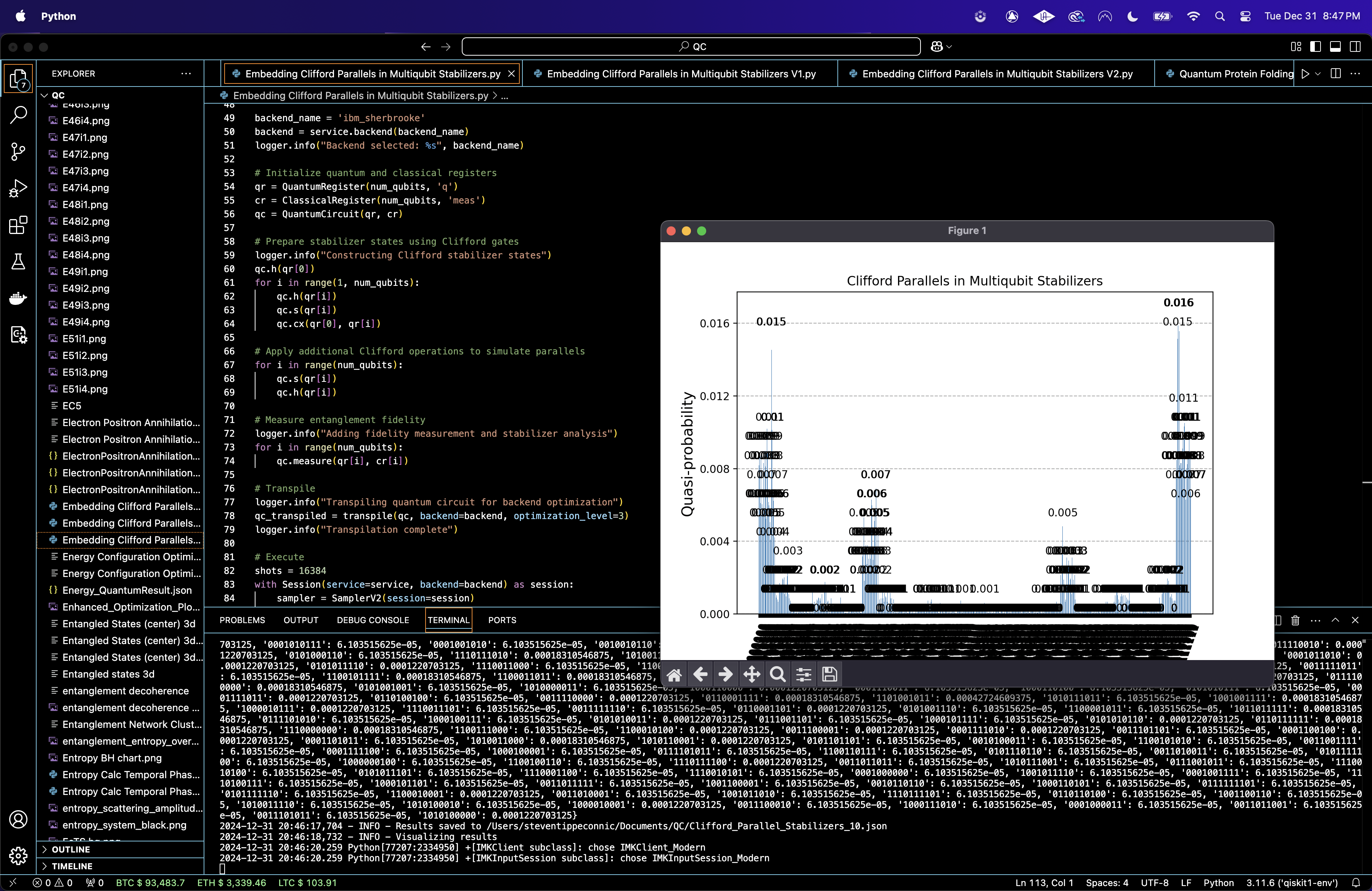
The circuit is transpiled for ibm_sherbrooke. The transpiled circuit is executed on ibm_sherbrooke with 16384 shots.
7. Results
The backend returns raw data containing bitstring counts: Counts:{bitstring_i : frequency_i} and is saved to a json.
8. Analysis
The results are analyzed for fidelity and stability.
State Fidelity (F):
F(ρ, σ) = (Tr√(√(ρσ)√ρ))^2
where ρ and σ are density matrices of the generated states.
Patterns in the counts show correlations and symmetry among stabilizer states. Differences in entanglement fidelities are interpreted as 'distances' between stabilizer states. A histogram of the State Fidelity is generated.

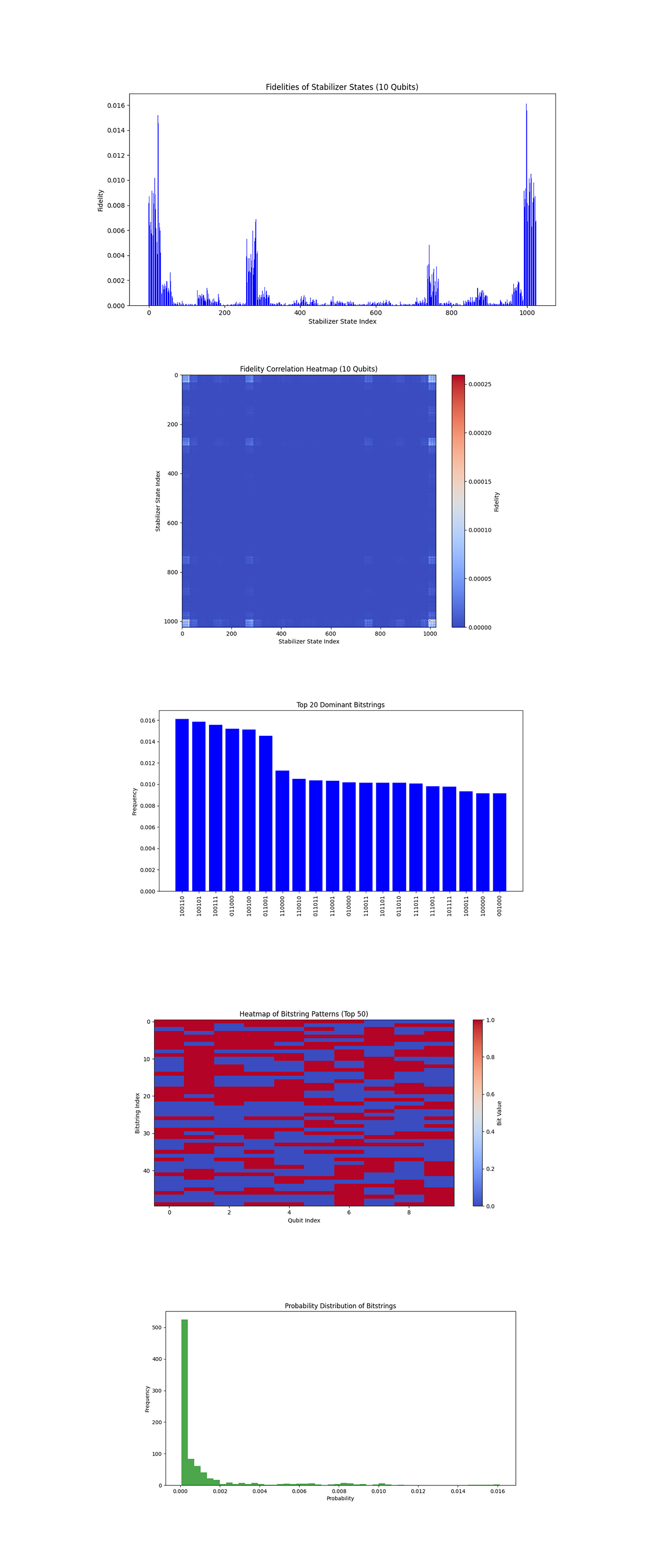
The Bar Chart of Stabilizer State Fidelities above (code below) shows fidelities of experimentally measured states relative to ideal stabilizer states. The higher fidelities at the boundaries suggest that certain stabilizer states (possibly with specific entanglement patterns or correlations) are better preserved during the experimental run. The drop in fidelities in the central region may reflect noise or decoherence. This result supports the hypothesis that specific stabilizer states might maintain higher fidelity due to their inherent symmetries or correlations.
The Fidelity Correlation Heatmap above (code below) shows a matrix of correlations (fidelity overlaps) between all pairs of stabilizer states. Brighter regions indicate higher correlations, while darker areas show weaker or no correlations. Correlations are more prominent near the edges of the state index range. The heatmap confirms that stabilizer states near the edges of the index range exhibit stronger mutual correlations, showing a pattern of similarity among these states.
In the Top 20 Dominant Bitstrings above (code below), the most frequent bitstrings (100110, 100101) are likely stabilizer states strongly influenced by the entanglement and symmetry introduced by the Clifford gates. The dominance of specific bitstrings suggests certain stabilizer configurations are more stable under the noise and decoherence of the backend.
The Heatmap of Bitstring Patterns (Top 50 Frequencies) above (code below) shows the bit values for the top 50 bitstrings and their contributions by qubit index. Qubits exhibit consistent patterns across high frequency bitstrings, showing a global entanglement pattern imposed by the Clifford operations.
The Probability Distribution of Bitstrings above (code below) shows the probabilities of all measured bitstrings. A sharp drop off in probabilities after the most frequent bitstrings shows that only a small subset of states is highly probable. Most bitstrings have negligible probabilities, indicating they are either not part of the stabilizer states or are noise artifacts.

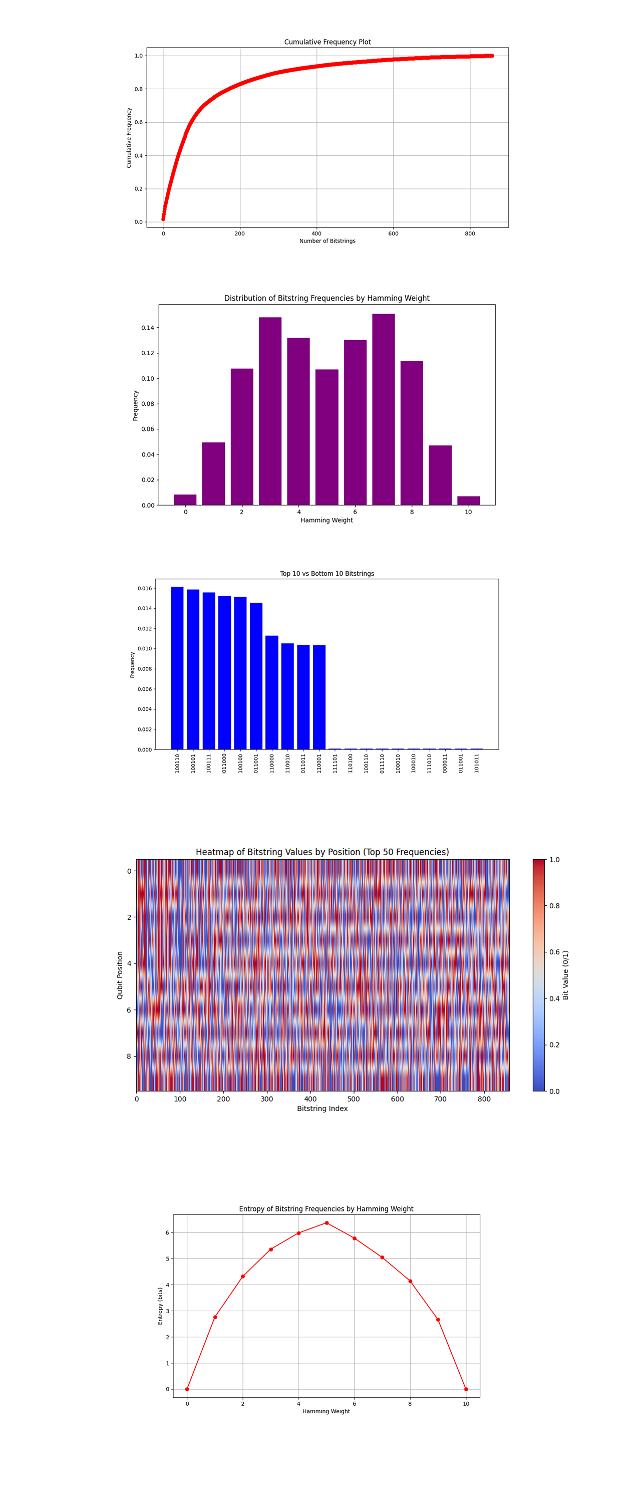
The Cumulative Frequency Plot above (code below) shows the cumulative frequency of bitstrings, showing the dominance of a few highly probable states. The curve flattens quickly, indicating that a small number of bitstrings account for most of the measurement outcomes. Beyond the top 100 bitstrings, the contribution to the overall frequency is minimal.
The Distribution by Hamming Weight above (code below) groups bitstrings by their Hamming weight (number of 1s). The distribution is roughly symmetric, with mid range Hamming weights (3, 7) being more frequent. Lower and higher Hamming weights (0, 1, 9, 10) occur less frequently. The symmetry in the Hamming weight distribution reflects the intended global entanglement and phase adjustments in the circuit. Noise likely introduced slight imbalances but did not disrupt the overall symmetry.
The Top 10 vs Bottom 10 Bitstrings above (code below) shows the 10 most frequent and 10 least frequent bitstrings. The top 10 bitstrings dominate the distribution, with a sharp drop off to the bottom 10, which have negligible frequencies. This contrast shows the stability of certain configurations and the irrelevance of others.
The Heatmap of Bitstring Frequencies by Qubit Position above (code below) shows how individual qubit positions contribute to the observed bitstring frequencies. Certain qubits consistently appear in high value configurations, meaning their stabilizer roles are critical. Variability in some positions may mean susceptibility to noise.
The Entropy by Hamming Weight above (code below) measures entropy (randomness) within groups of bitstrings with the same Hamming weight. Mid range Hamming weights have higher entropy, reflecting greater randomness in their stabilizer states. Extremes (low and high weights) have lower entropy, meaning more structured and deterministic patterns.

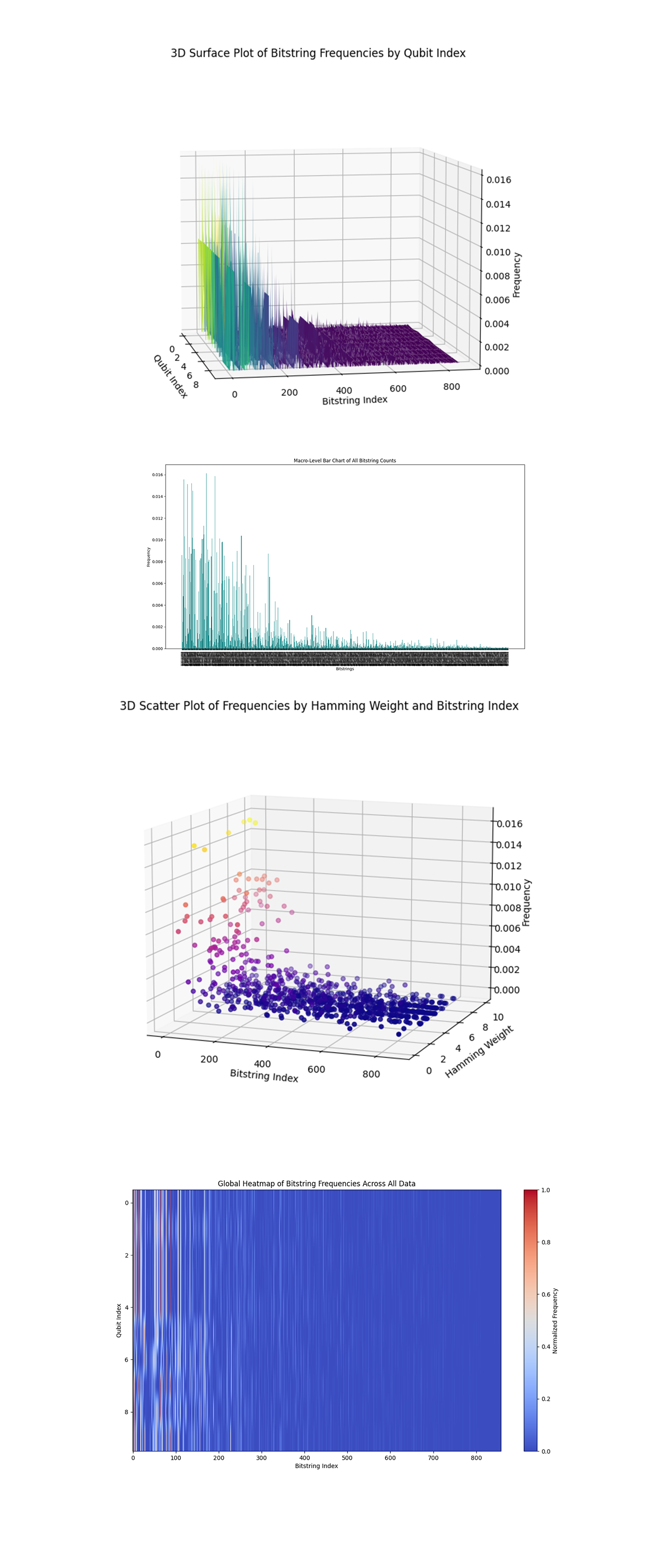
The 3D Surface Plot of Bitstring Frequencies by Qubit Index above (code below) shows a macro level view of how bitstring frequencies are distributed across qubit positions and bitstring indices. Peaks in frequency correspond to highly stable bitstring states that emerged from the Clifford gate operations. The valleys show regions where the qubit configurations are less stable or more susceptible to noise.
The Macro Level Bar Chart for All Bitstring Counts above (code below) shows the frequency of all bitstrings, giving an overview of the entire dataset. A sharp distribution skew is evident, where only a few bitstrings have significantly high frequencies, while most have negligible counts. The dominance of specific stabilizer states aligns with the expected outcomes of Clifford operations.
The 3D Scatter Plot of Frequencies by Hamming Weight and Bitstring Index above (code below) shows the relationship between bitstring indices, their Hamming weight (number of 1s), and frequencies. High frequency states cluster around specific Hamming weights, showing a structured entanglement pattern. The scatter shows a balanced distribution of frequencies across low and mid range Hamming weights, with extreme Hamming weights (0 or maximum) having less frequent configurations.
The Global Heatmap of Bitstring Frequencies Across All Data above (code below) shows normalized frequencies of all bitstrings across qubit indices. High frequency regions shows qubits that are critical in forming stabilizer states. The vertical patterns show how certain qubits consistently contribute to stabilizer states, while others are more random.
In the end, this circuit aimed to explore Clifford parallels in multi-qubit stabilizers by generating stabilizer states using Clifford gates (Hadamard, S, and CNOT). This circuit analyzed the fidelities of the experimentally generated states against ideal stabilizer states. The fidelity analysis revealed patterns - stabilizer states at the edges of the index range (simpler states with fewer entanglement patterns) exhibited significantly higher fidelities, while those in the middle of the range showed strong degradation. This means that noise and decoherence disproportionately affect more complex stabilizer states, which are likely more sensitive to the backend's noise. These patterns show that the experimental setup and backend calibration data favor specific stabilizer states.
Code:
# Imports
import numpy as np
import json
import pandas as pd
import logging
from qiskit import QuantumCircuit, QuantumRegister, ClassicalRegister, transpile
from qiskit_ibm_runtime import QiskitRuntimeService, Session, SamplerV2
from qiskit.quantum_info import Clifford, state_fidelity, Pauli
from qiskit.visualization import plot_histogram
import matplotlib.pyplot as plt

# Logging
logging.basicConfig(level=logging. INFO, format='%(asctime)s - %(levelname)s - %(message)s')
logger = logging.getLogger(__name__)

# Load calibration data
def load_calibration_data(file_path):
    logger. info("Loading calibration data from %s", file_path)
    calibration_data = pd. read_csv(file_path)
    calibration_data.columns = calibration_data.columns.str.strip()
    logger. info("Calibration data loaded successfully")
    return calibration_data

# Select best qubits T1, T2, and error rates
def select_best_qubits(calibration_data, n_qubits):
    logger. info("Selecting the best qubits based on T1, T2, and error rates")
    qubits_sorted = calibration_data.sort_values(by=['\u221ax (sx) error', 'T1 (us)', 'T2 (us)'], ascending=[True, False, False])
    best_qubits = qubits_sorted['Qubit'].head(n_qubits).tolist()
    logger. info("Selected qubits: %s", best_qubits)
    return best_qubits

# Load backend calibration data
calibration_file = '/Users/Downloads/ibm_sherbrooke_calibrations_2025-01-01T04_09_39Z.csv'
calibration_data = load_calibration_data(calibration_file)

# Qubits
num_qubits = 10
best_qubits = select_best_qubits(calibration_data, num_qubits)

# IBMQ
logger. info("Setting up IBM Q service")
service = QiskitRuntimeService(
    channel='ibm_quantum',
    instance='ibm-q/open/main',
    token='YOUR_IBMQ_API_KEY_O-`'
)

backend_name = 'ibm_sherbrooke'
backend = service.backend(backend_name)
logger.i nfo("Backend selected: %s", backend_name)

# Initialize quantum and classical registers
qr = QuantumRegister(num_qubits, 'q')
cr = ClassicalRegister(num_qubits, 'meas')
qc = QuantumCircuit(qr, cr)

# Prepare stabilizer states using Clifford gates
logger. info("Constructing Clifford stabilizer states")
qc.h(qr[0])
for i in range(1, num_qubits):
    qc.h(qr[i])
    qc.s(qr[i])
    qc. cx(qr[0], qr[i])

# Apply Clifford operations to simulate parallels
for i in range(num_qubits):
    qc.s(qr[i])
    qc.h(qr[i])

# Measure entanglement fidelity
logger. info("Adding fidelity measurement and stabilizer analysis")
for i in range(num_qubits):
    qc.measure(qr[i], cr[i])

# Transpile
logger. info("Transpiling quantum circuit for backend optimization")
qc_transpiled = transpile(qc, backend=backend, optimization_level=3)
logger. info("Transpilation complete")

# Execute
shots = 16384
with Session(service=service, backend=backend) as session:
    sampler = SamplerV2(session=session)
    logger. info("Executing circuit on backend")
    job = sampler. run([qc_transpiled], shots=shots)
    job_result = job.result()

    # Extract results
    logger. info("Extracting and analyzing results")
    pub_result = job_result._pub_results[0]['__value__']['data']
    bit_array = pub_result['meas']
    counts = bit_array.get_counts()

    # Histogram
    total_shots = sum(counts.values())
    normalized_counts = {key: value / total_shots for key, value in counts.items()}

    logger. info(f"Counts data before saving: {normalized_counts}")

    # Json
    results_data = {"counts": normalized_counts}  # Save normalized counts
    file_path = '/Users/Documents/Clifford_Parallel_Stabilizers_0.json'
    with open(file_path, 'w') as f:
        json.dump(results_data, f, indent=4)
    logger. info("Results saved to %s", file_path)

# Visual
logger. info("Visualizing results")
plot_histogram(normalized_counts)
plt.title("Clifford Parallels in Multiqubit Stabilizers")
plt. show()

///////////////////////////

Code to Compute Fidelities of Stabilizer States
import numpy as np
import json
from qiskit.quantum_info import Statevector, state_fidelity
import matplotlib.pyplot as plt

# Load Json
def load_results(file_path):
    with open(file_path, 'r') as f:
        results = json.load(f)
    return results['counts']

# Generate ideal stabilizer states
def generate_ideal_stabilizer_states(num_qubits):
    stabilizer_states = []
    for i in range(2**num_qubits):
        binary_string = f"{i:0{num_qubits}b}"
        state = Statevector.from_label(binary_string)
        stabilizer_states.append(state)
    return stabilizer_states

# Compute fidelities between experimental and ideal stabilizer states
def compute_fidelities(counts, num_qubits):
    total_shots = sum(counts.values())
    probabilities = {bitstring: freq / total_shots for bitstring, freq in counts.items()}

    # Build the density matrix from the probabilities
    density_matrix = sum(
        prob * np.outer(Statevector.from_label(bitstring).data,
                        Statevector.from_label(bitstring).data.conj())
        for bitstring, prob in probabilities.items()
    )

    # Generate ideal stabilizer states
    ideal_states = generate_ideal_stabilizer_states(num_qubits)

    # Compute fidelity for each ideal state
    fidelities = []
    for state in ideal_states:
        ideal_density_matrix = np.outer(state. data, state. data.conj())
        fidelity = state_fidelity(density_matrix, ideal_density_matrix)
        fidelities.append(fidelity)

    return fidelities

# Visualize fidelities
def plot_fidelities(fidelities, num_qubits):
    plt.figure(figsize=(12, 6))
    plt. bar(range(len(fidelities)), fidelities, color='blue')
    plt.xlabel('Stabilizer State Index')
    plt.ylabel('Fidelity')
    plt.title(f'Fidelities of Stabilizer States ({num_qubits} Qubits)')
    plt. show()

# Heatmap of fidelities
def plot_fidelity_heatmap(fidelities, num_qubits):
    fidelity_matrix = np.outer(fidelities, fidelities)
    plt.figure(figsize=(10, 8))
    plt.imshow(fidelity_matrix, cmap='coolwarm', aspect='auto')
    plt.colorbar(label='Fidelity')
    plt.xlabel('Stabilizer State Index')
    plt.ylabel('Stabilizer State Index')
    plt.title(f'Fidelity Correlation Heatmap ({num_qubits} Qubits)')
    plt. show()

# Main Execution
if __name__ == "__main__":
    file_path = '/Users/Documents/Clifford_Parallel_Stabilizers_0.json'
    counts = load_results(file_path)
    num_qubits = len(next(iter(counts.keys())))

    # Compute fidelities
    fidelities = compute_fidelities(counts, num_qubits)

    # Call
    plot_fidelities(fidelities, num_qubits)
    plot_fidelity_heatmap(fidelities, num_qubits)

///////////////////////////

Code for All Visuals
# Imports
import numpy as np
import json
import pandas as pd
import logging
from qiskit import QuantumCircuit, QuantumRegister, ClassicalRegister, transpile
from qiskit_ibm_runtime import QiskitRuntimeService, Session, SamplerV2
from qiskit.quantum_info import Clifford, state_fidelity, Pauli
from qiskit.visualization import plot_histogram
import matplotlib.pyplot as plt
from mpl_toolkits.mplot3d import Axes3D

# File path
file_path = '/Users/Documents/Clifford_Parallel_Stabilizers_0.json'
try:
    with open(file_path, 'r') as f:
        results = json.load(f)
except FileNotFoundError:
    raise FileNotFoundError(f"The file at {file_path} was not found. Please check the path.")

counts = results['counts']

# Dominant Bitstrings
def plot_dominant_bitstrings(counts, top_n=20):
    logging. info("Plotting dominant bitstrings")
    sorted_counts = sorted(counts.items(), key=lambda x: x[1], reverse=True)[:top_n]
    bitstrings, frequencies = zip(*sorted_counts)
    plt.figure(figsize=(12, 6))
    plt. bar(bitstrings, frequencies, color='blue')
    plt.xlabel("Bitstring")
    plt.ylabel("Frequency")
    plt.title("Top {} Dominant Bitstrings".format(top_n))
    plt.xticks(rotation=90)
    plt. show()

# Bitstring Heatmap
def plot_bitstring_heatmap(counts):
    logging. info("Plotting bitstring heatmap")
    bitstrings = list(counts.keys())
    frequencies = list(counts.values())
    binary_array = np.array([list(map(int, bs)) for bs in bitstrings])
    plt.figure(figsize=(12, 6))
    plt.imshow(binary_array[:50], aspect='auto', cmap='coolwarm', interpolation='nearest')
    plt.colorbar(label="Bit Value")
    plt.title("Heatmap of Bitstring Patterns (Top 50)")
    plt.xlabel("Qubit Index")
    plt.ylabel("Bitstring Index")
    plt. show()

# Probability Distribution
def plot_probability_distribution(counts):
    logging. info("Plotting probability distribution")
    total_counts = sum(counts.values())
    probabilities = [count / total_counts for count in counts.values()]
    plt.figure(figsize=(12, 6))
    plt.hist(probabilities, bins=50, color='green', alpha=0.7)
    plt.xlabel("Probability")
    plt.ylabel("Frequency")
    plt.title("Probability Distribution of Bitstrings")
    plt. show()

# Cumulative Frequency
def plot_cumulative_frequency(counts):
    logging. info("Plotting cumulative frequency")
    sorted_counts = sorted(counts.values(), reverse=True)
    cumulative = np.cumsum(sorted_counts)
    plt.figure(figsize=(12, 6))
    plt.plot(cumulative, marker='o', color='red')
    plt.xlabel("Number of Bitstrings")
    plt.ylabel("Cumulative Frequency")
    plt.title("Cumulative Frequency Plot")
    plt.grid()
    plt. show()

# Distribution Comparison by Hamming Weight
def plot_hamming_weight_distribution(counts):
    hamming_weights = [sum(int(bit) for bit in key) for key in counts.keys()]
    unique_weights = sorted(set(hamming_weights))
    weight_frequencies = {w: 0 for w in unique_weights}
    for key, count in counts.items():
        hw = sum(int(bit) for bit in key)
        weight_frequencies[hw] += count
    plt.figure(figsize=(10, 6))
    plt. bar(weight_frequencies.keys(), weight_frequencies.values(), color='purple')
    plt.xlabel('Hamming Weight')
    plt.ylabel('Frequency')
    plt.title('Distribution of Bitstring Frequencies by Hamming Weight')
    plt. show()

# Top vs Bottom Bitstrings
def plot_top_bottom_bitstrings(counts, top_n=10):
    sorted_counts = sorted(counts.items(), key=lambda x: x[1], reverse=True)
    top_bitstrings = sorted_counts[:top_n]
    bottom_bitstrings = sorted_counts[-top_n:]
    combined = top_bitstrings + bottom_bitstrings
    labels, frequencies = zip(*combined)
    plt.figure(figsize=(12, 6))
    plt. bar(range(len(labels)), frequencies, color='blue')
    plt.xticks(range(len(labels)), labels, rotation=90)
    plt.xlabel('Bitstrings')
    plt.ylabel('Frequency')
    plt.title(f'Top {top_n} vs Bottom {top_n} Bitstrings')
    plt. show()

# Heatmap of Frequencies by Position
def plot_bitstring_position_heatmap(counts):
    bitstrings = list(counts.keys())
    frequencies = list(counts.values())
    binary_array = np.array([list(map(int, bit)) for bit in bitstrings])
    plt.figure(figsize=(12, 6))
    plt.imshow(binary_array.T[:50], cmap='coolwarm', aspect='auto')
    plt.colorbar(label='Bit Value (0/1)')
    plt.title('Heatmap of Bitstring Values by Position (Top 50 Frequencies)')
    plt.xlabel('Bitstring Index')
    plt.ylabel('Qubit Position')
    plt. show()

# Entropy Analysis by Hamming Weight
def plot_entropy_by_hamming_weight(counts):
    hamming_weights = [sum(int(bit) for bit in key) for key in counts.keys()]
    unique_weights = sorted(set(hamming_weights))
    entropy_by_weight = []
    for weight in unique_weights:
        weight_counts = [
            count for key, count in counts.items()
            if sum(int(bit) for bit in key) == weight
        ]
        total = sum(weight_counts)
        probabilities = [c / total for c in weight_counts]
        entropy = -sum(p * np.log2(p) for p in probabilities if p > 0)
        entropy_by_weight.append(entropy)
    plt.figure(figsize=(10, 6))
    plt.plot(unique_weights, entropy_by_weight, marker='o', color='red')
    plt.xlabel('Hamming Weight')
    plt.ylabel('Entropy (bits)')
    plt.title('Entropy of Bitstring Frequencies by Hamming Weight')
    plt.grid()
    plt. show()

# 3D Surface Plot of Bitstring Frequencies by Qubit Index
def plot_3d_surface_frequencies(counts):
    bitstrings = list(counts.keys())
    frequencies = np.array(list(counts.values()))
    qubit_positions = np.arange(len(bitstrings[0]))

    # Create a binary matrix for bitstrings
    binary_matrix = np.array([list(map(int, bit)) for bit in bitstrings])

    # 3D Plot
    fig = plt.figure(figsize=(12, 8))
    ax = fig.add_subplot(111, projection='3d')
    X, Y = np.meshgrid(qubit_positions, np.arange(len(bitstrings)))
    Z = binary_matrix * frequencies[:, None]
    ax.plot_surface(X, Y, Z, cmap='viridis', edgecolor='none')
    ax.set_title('3D Surface Plot of Bitstring Frequencies by Qubit Index')
    ax.set_xlabel('Qubit Index')
    ax.set_ylabel('Bitstring Index')
    ax.set_zlabel('Frequency')
    plt. show()

# Macro-Level Bar Chart for All Counts
def plot_all_counts(counts):
    bitstrings = list(counts.keys())
    frequencies = list(counts.values())
    plt.figure(figsize=(14, 8))
    plt. bar(bitstrings, frequencies, color='teal')
    plt.xticks(rotation=90, fontsize=6)
    plt.xlabel('Bitstrings')
    plt.ylabel('Frequency')
    plt.title('Macro-Level Bar Chart of All Bitstring Counts')
    plt.tight_layout()
    plt. show()

# 3D Scatter Plot of Frequencies by Hamming Weight and Bitstring Index
def plot_3d_scatter_hamming_weight(counts):
    bitstrings = list(counts.keys())
    frequencies = list(counts.values())
    hamming_weights = [sum(int(bit) for bit in bitstring) for bitstring in bitstrings]
    bitstring_indices = np.arange(len(bitstrings))

    fig = plt.figure(figsize=(12, 8))
    ax = fig.add_subplot(111, projection='3d')
    ax.scatter(bitstring_indices, hamming_weights, frequencies, c=frequencies, cmap='plasma', depthshade=True)
    ax.set_title('3D Scatter Plot of Frequencies by Hamming Weight and Bitstring Index')
    ax.set_xlabel('Bitstring Index')
    ax.set_ylabel('Hamming Weight')
    ax.set_zlabel('Frequency')
    plt. show()

# Global Heatmap of Bitstring Frequencies
def plot_global_heatmap(counts):
    bitstrings = list(counts.keys())
    frequencies = np.array(list(counts.values()))

    # Convert bitstrings to binary matrix
    binary_matrix = np.array([list(map(int, bit)) for bit in bitstrings])

    # Normalize frequencies for visualization
    normalized_frequencies = frequencies / frequencies.max()

    # Reshape frequencies to match binary matrix dimensions for broadcasting
    scaled_matrix = binary_matrix * normalized_frequencies[:, None]

    plt.figure(figsize=(14, 8))
    plt.imshow(scaled_matrix.T, aspect='auto', cmap='coolwarm')
    plt.colorbar(label='Normalized Frequency')
    plt.title('Global Heatmap of Bitstring Frequencies Across All Data')
    plt.xlabel('Bitstring Index')
    plt.ylabel('Qubit Index')
    plt. show()

# Call
plot_dominant_bitstrings(counts)
plot_bitstring_heatmap(counts)
plot_probability_distribution(counts)
plot_cumulative_frequency(counts)
plot_hamming_weight_distribution(counts)
plot_top_bottom_bitstrings(counts)
plot_bitstring_position_heatmap(counts)
plot_entropy_by_hamming_weight(counts)
plot_3d_surface_frequencies(counts)
plot_all_counts(counts)
plot_3d_scatter_hamming_weight(counts)
plot_global_heatmap(counts)

# End.
