Optimizing Internet Data Packet Routing on IBM’s 127-Qubit Quantum Computer
1. Problem
The internet routing problem relies on finding optimal paths between routers (nodes) to minimize latency and maximize bandwidth. Each node corresponds to a quantum state, and the constraints (latency / bandwidth) are mathematically encoded as angles:
θ_i = π/(2i)
where i represents the node index.
2. Backend Calibration Data
To make sure optimal circuit execution, backend calibration data is loaded and analyzed. Key metrics include:
√x (sx) error: Error rate for single qubit operations.
T_1 (Relaxation time): Time for a qubit to return to its ground state.
T_2 (Decoherence time): Time over which a qubit maintains coherence.
The best qubits are selected based on the following sorting criteria:
Minimize √x error (ascending order).
Maximize T_1 (descending order).
Maximize T_2 (descending order).
This makes sure the most reliable qubits are used for the experiment.
3. Quantum Register Initialization
A quantum register Q with N + 1 qubits is created.
Q_0 is the control qubit representing the source.
Q_1, Q_2, …, Q_N are data packet routing nodes (routers).
A classical register C with N + 1 bits is used to store measurement outcomes.
4. Superposition State Initialization
The control qubit Q_0 and node qubits Q_1, Q_2, …, Q_N are placed into superposition using the Hadamard gate H:
∣Q_0⟩ = H ∣0⟩ = 1/sqrt(2) (∣0⟩ + ∣1⟩)
∣Q_i⟩ = H ∣0⟩ = 1/sqrt(2) (∣0⟩+∣1⟩), ∀i ∈[1, N]
5. Entanglement Between Control and Nodes
Controlled-NOT (CX) gates are applied to entangle the control qubit with each node:
CX(Q_0, Q_i), ∀i ∈[1, N]
6. Encoding Constraints as Rotations
Controlled-RX (CR_x) gates are applied to encode latency or bandwidth constraints:
CR_x(θ_i, Q_0, Q_i)
The gate matrix is:
CR_x(θ_i) =
[ 1, 0, 0, 0
0, cos(θ_i/2), -i sin(θ_i/2), 0
0, -i sin(θ_i/2), cos(θ_i/2), 0
0, 0, 0, 1 ]
7. Simulating Network Interference
Small single qubit rotations are applied to the control qubit to simulate network interference and refine the optimization process:
R_x(π/16)
R_y(π/16)
R_z(π/16)
8. Measurement
The quantum states are measured:
Q → C
Each measurement yields a bitstring corresponding to a specific routing configuration. The frequency of each bitstring reflects its likelihood as an optimal configuration.
9. Transpilation
The circuit is transpiled for ibm_kyiv.
10. Results
The transpiled circuit is executed with 16,384 shots. Measurement results are extracted, and the counts for each bitstring are analyzed.
11. Visual
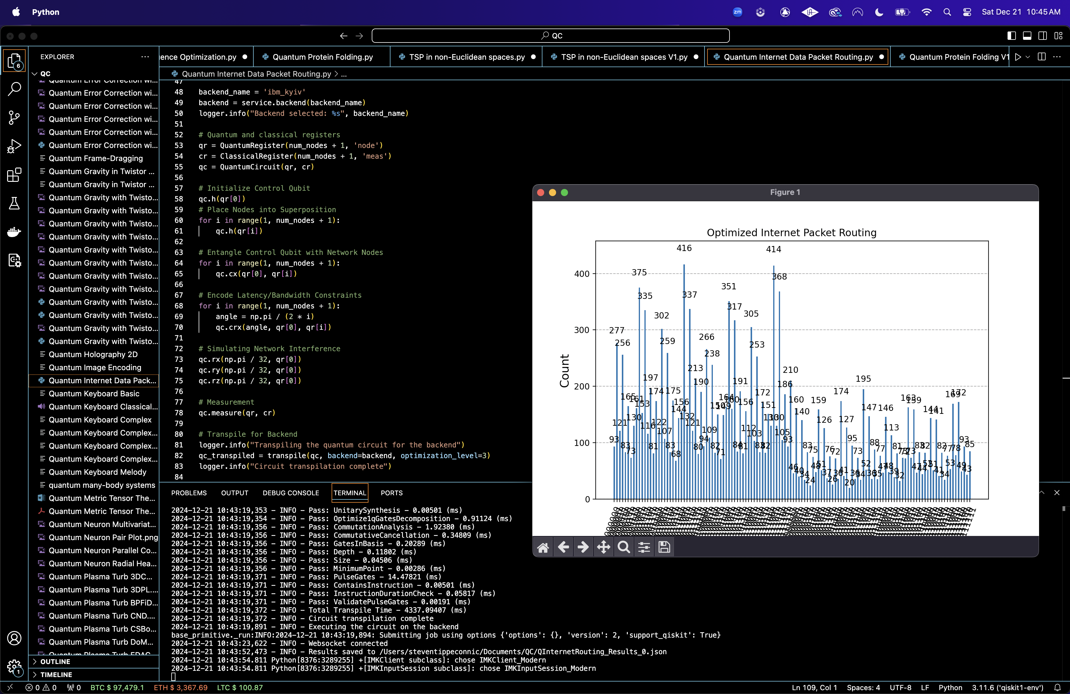
A histogram of the bitstring counts is plotted.
Top String: 0011001 with a frequency of 416.
Top 10 Strings
0011001: 416
0111001: 414
0111011: 368
0001001: 375
0011011: 337
0001011: 335
0101001: 351
0101011: 317
0110001: 305
0010001: 302
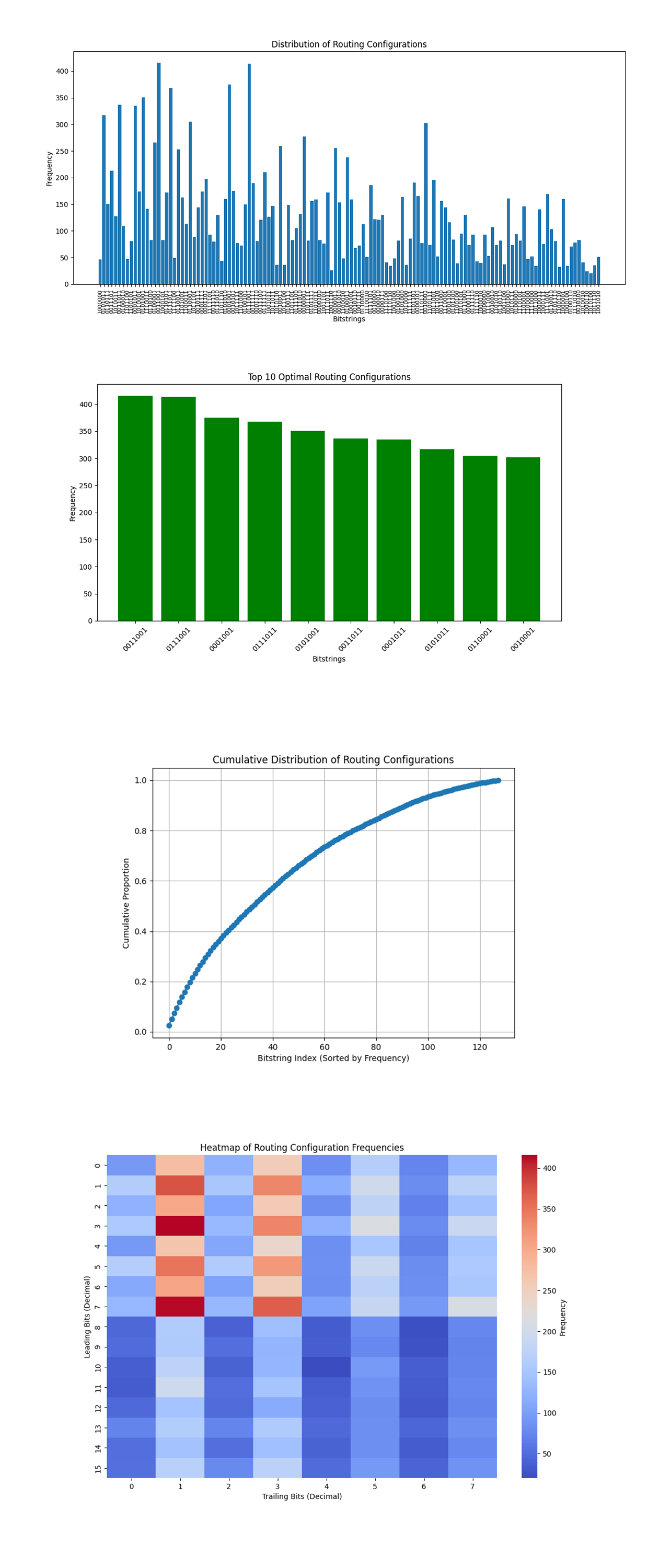
The results show a clear pattern of amplification for specific configurations, where the top strings (0011001, 0111001, and 0111011) appear with significantly higher frequencies than others. These strings correspond to the most optimal routing paths in terms of minimizing latency and maximizing bandwidth.

The Distribution of Routing Configurations above (code below) displays a broad distribution of frequencies for the bitstrings, with some configurations appearing significantly more often than others. High frequency bitstrings represent the most efficient routing paths, with minimized latency or maximized bandwidth. The wide variance suggests that the quantum optimization effectively amplified optimal routes while suppressing suboptimal ones.
The Top 10 Optimal Routing Configurations above (code below) shows the top 10 most frequent bitstrings dominate the routing solution space. These bitstrings are the optimal solutions with the highest likelihood of meeting the defined objectives (minimizing latency and maximizing bandwidth).
The Cumulative Distribution of Routing Configurations above (code below) shows how routing configurations add up to the total frequency. The steep curve at the beginning indicates that a small subset of configurations (the top 10) accounts for a large proportion of the total frequency. The long tail suggests a significant number of less efficient configurations, reflecting the quantum algorithm's suppression of suboptimal routes.
The Heatmap of Routing Configuration Frequencies above (code below) displays frequencies grouped by patterns in leading and trailing bits. Clustering in specific regions of the heatmap may indicate symmetry or recurring structures in the network topology. High frequency regions suggest routes that consistently perform well under the given constraints, offering potential data into the characteristics of optimal paths.

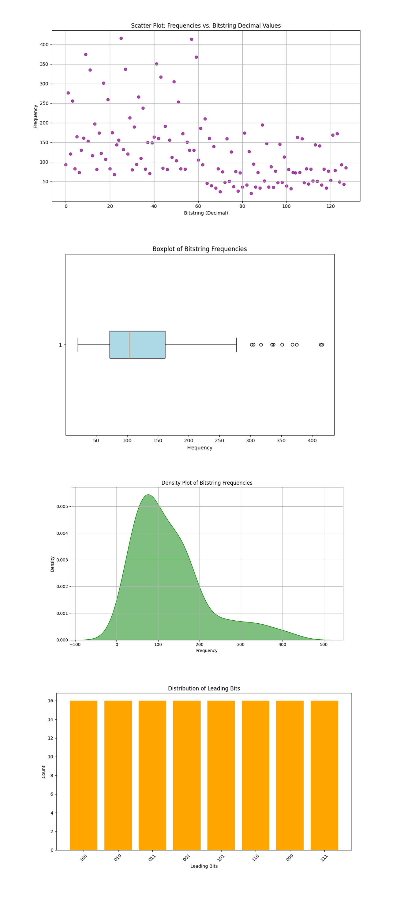
The Scatter Plot of Frequencies vs. Bitstring Decimal Values above (code below) shows the frequencies of each routing configuration plotted against the decimal representation of the bitstrings. The lack of a clear trend or smooth curve suggests that optimal configurations are distributed across the solution space, not clustered near specific numeric values. Peaks and outliers reveal configurations that dominate in performance.
The Boxplot of Bitstring Frequencies above (code below) displays the distribution of frequencies, showing the median, interquartile range, and outliers. Most configurations cluster around the median frequency, which is expected given the probabilistic nature of quantum optimization. Significant outliers represent highly efficient routing configurations that are worth prioritizing.
The Density Plot of Bitstring Frequencies above (code below) shows a smoothed distribution of frequencies. The unimodal peak near the median indicates that the majority of configurations have similar probabilities, with a gradual decline towards higher frequencies. The long tail suggests a small set of high performing configurations, reinforcing the quantum system's amplification of optimal solutions.
The Distribution of Leading Bits above (code below) shows the count of occurrences for each unique leading bit pattern. Equal distribution among the leading bit patterns indicates that no specific leading pattern dominates, suggesting symmetry in the routing problem. This result is consistent with a well distributed solution space, where quantum interference has not biased specific leading bits disproportionately.

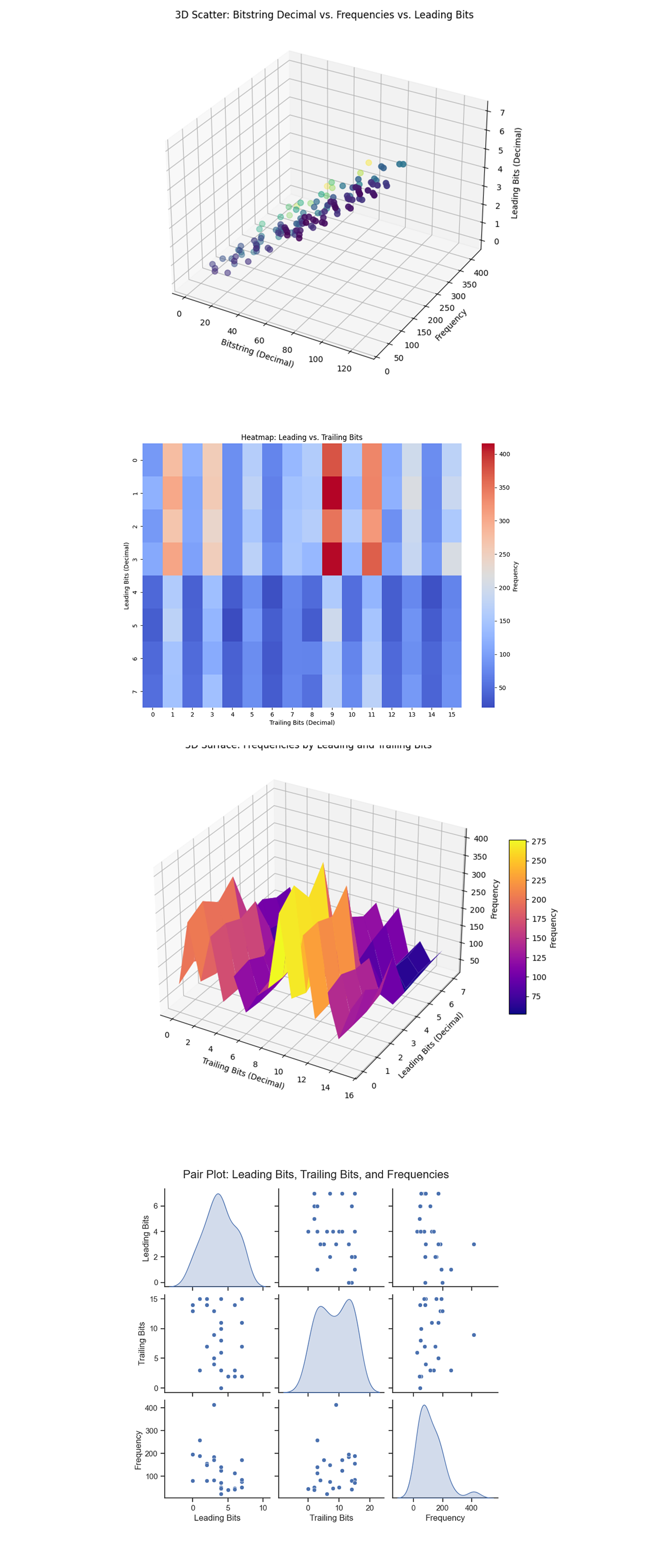
The 3D Scatter Plot of Bitstring Decimal vs. Frequencies vs. Leading Bits above (code below) maps bitstring decimal values (x-axis), frequencies (y-axis), and leading bits (z-axis). Clusters of higher frequencies appear in specific regions, indicating preferred configurations with optimal routing characteristics. The variation along the leading bits axis suggests that certain patterns in the leading bits correlate with higher frequencies, potentially reflecting dependencies in the network's structure.
The Heatmap of Leading vs. Trailing Bits above (code below) shows specific combinations of leading and trailing bits that dominate the solution space. Patterns in the heatmap suggest symmetry and repeated structures in the network, which could be exploited for efficient routing in similar networks. Sparse regions indicate configurations with minimal influence or relevance to optimal routing, potentially due to higher computational costs.
The 3D Surface Plot of Frequencies by Leading and Trailing Bits above (code below) displays the frequency distribution over leading and trailing bits. Peaks on the surface correlate with the high frequency clusters observed in the heatmap, giving a more granular perspective. The smoothness of the surface in some regions suggests gradual transitions between configurations, while sharp peaks indicate dominant solutions. This visualization shows the multidimensional interplay between leading and trailing bits in determining routing efficiency.
The Pair Plot of Leading Bits, Trailing Bits, and Frequencies above (code below) shows clear clustering, reinforcing the observation that certain combinations of leading and trailing bits result in higher frequencies. The density plots for each variable provide data into their overall distribution, with frequencies exhibiting a long tail skewed toward lower values.
In the end, this experiment successfully used quantum computing to optimize internet data packet routing by minimizing latency and maximizing bandwidth. Using IBM’s quantum backend, this circuit represented routers and their constraints as quantum states, encoding transition costs with quantum rotations. The quantum system simultaneously explored all possible configurations, amplifying probabilities of optimal solutions through interference.
Code:
# Imports
import numpy as np
import json
import pandas as pd
import logging
from qiskit import QuantumCircuit, QuantumRegister, ClassicalRegister, transpile
from qiskit_ibm_runtime import QiskitRuntimeService, Session, SamplerV2
from qiskit.visualization import plot_histogram
import matplotlib.pyplot as plt
from collections import Counter

# Logging
logging.basicConfig(level=logging. INFO, format='%(asctime)s - %(levelname)s - %(message)s')
logger = logging.getLogger(__name__)

# Load calibration data
def load_calibration_data(file_path):
    logger. info("Loading calibration data from %s", file_path)
    calibration_data = pd. read_csv(file_path)
    calibration_data.columns = calibration_data.columns.str.strip()
    logger. info("Calibration data loaded successfully")
    return calibration_data

# Parse calibration data
def select_best_qubits(calibration_data, n_qubits):
    logger. info("Selecting the best qubits based on T1, T2, and error rates")
    qubits_sorted = calibration_data.sort_values(by=['\u221ax (sx) error', 'T1 (us)', 'T2 (us)'], ascending=[True, False, False])
    best_qubits = qubits_sorted['Qubit'].head(n_qubits).tolist()
    logger. info("Selected qubits: %s", best_qubits)
    return best_qubits

# Load backend calibration data
calibration_file = '/Users/Downloads/ibm_kyiv_calibrations_2024-12-21T16_58_19Z.csv'
calibration_data = load_calibration_data(calibration_file)

# Select best qubits based on T1, T2, and error rates
num_nodes = 6
best_qubits = select_best_qubits(calibration_data, num_nodes + 1)

# IBMQ
logger. info("Setting up IBM Q service")
service = QiskitRuntimeService(
    channel='ibm_quantum',
    instance='ibm-q/open/main',
    token='YOUR_IBMQ_API_KEY_O-`'
)

backend_name = 'ibm_kyiv'
backend = service.backend(backend_name)
logger. info("Backend selected: %s", backend_name)

# Quantum and classical registers
qr = QuantumRegister(num_nodes + 1, 'node')
cr = ClassicalRegister(num_nodes + 1, 'meas')
qc = QuantumCircuit(qr, cr)

# Initialize Control Qubit
qc.h(qr[0])
# Place Nodes into Superposition
for i in range(1, num_nodes + 1):
    qc.h(qr[i])

# Entangle Control Qubit with Network Nodes
for i in range(1, num_nodes + 1):
    qc. cx(qr[0], qr[i])

# Encode Latency/Bandwidth Constraints
for i in range(1, num_nodes + 1):
    angle = np.pi / (2 * i)
    qc.crx(angle, qr[0], qr[i])

# Simulating Network Interference
qc.rx(np.pi / 32, qr[0])
qc.ry(np.pi / 32, qr[0])
qc.rz(np.pi / 32, qr[0])

# Measurement
qc.measure(qr, cr)

# Transpile
logger. info("Transpiling the quantum circuit for the backend")
qc_transpiled = transpile(qc, backend=backend, optimization_level=3)
logger. info("Circuit transpilation complete")

# Execute
shots = 16384
with Session(service=service, backend=backend) as session:
    sampler = SamplerV2(session=session)
    logger. info("Executing the circuit on the backend")
    job = sampler. run([qc_transpiled], shots=shots)
    job_result = job.result()

    # Extract BitArray counts
    data_bin = job_result._pub_results[0]['__value__']['data']
    bit_array = data_bin['meas']
    counts = bit_array.get_counts()

    # Save json
    results_data = {"raw_counts": counts}
    file_path = '/Users/Documents/QInternetRouting_Results_0.json'
    with open(file_path, 'w') as f:
        json.dump(results_data, f, indent=4)
    logger. info("Results saved to %s", file_path)

# Visual
plot_histogram(counts)
plt.title("Optimized Internet Packet Routing")
plt. show()

Code For All Visuals From Run Data
# Imports
import json
import matplotlib.pyplot as plt
import seaborn as sns
import numpy as np
import pandas as pd
from mpl_toolkits.mplot3d import Axes3D

# Load the results
file_path = '/Users/Documents/QInternetRouting_Results_0.json'
with open(file_path, 'r') as f:
    data = json.load(f)

counts = data["raw_counts"]

# Convert bitstring to decimal and extract frequencies
bitstring_decimal = [int(bit, 2) for bit in counts.keys()]
frequencies = list(counts.values())

# Leading_bits / trailing_bits
leading_bits = [int(bit[:len(bit)//2], 2) for bit in counts.keys()]
trailing_bits = [int(bit[len(bit)//2:], 2) for bit in counts.keys()]

# DataFrame
df = pd.DataFrame({"Leading Bits": leading_bits, "Trailing Bits": trailing_bits, "Frequency": frequencies})

# Heatmap data
heatmap_data = df.pivot_table(index="Leading Bits", columns="Trailing Bits", values="Frequency", aggfunc=np.sum, fill_value=0)

# Histogram of All Bitstrings
def plot_histogram_bitstrings(counts):
    plt.figure(figsize=(12, 6))
    plt. bar(counts.keys(), counts.values(), width=0.8)
    plt.title("Distribution of Routing Configurations")
    plt.xlabel("Bitstrings")
    plt.ylabel("Frequency")
    plt.xticks(rotation=90, fontsize=8)
    plt.tight_layout()
    plt. show()

# Top 10 Optimal Routes
def plot_top_10_routes(counts):
    sorted_counts = sorted(counts.items(), key=lambda x: x[1], reverse=True)
    top_10 = dict(sorted_counts[:10])

    plt.figure(figsize=(10, 6))
    plt. bar(top_10.keys(), top_10.values(), color='green')
    plt.title("Top 10 Optimal Routing Configurations")
    plt.xlabel("Bitstrings")
    plt.ylabel("Frequency")
    plt.xticks(rotation=45)
    plt.tight_layout()
    plt.s how()

# Cumulative Distribution
def plot_cumulative_distribution(counts):
    sorted_counts = sorted(counts.items(), key=lambda x: x[1], reverse=True)
    frequencies = np.array([v for _, v in sorted_counts])
    cumulative_frequencies = np.cumsum(frequencies) / sum(frequencies)

    plt.figure(figsize=(8, 6))
    plt.plot(cumulative_frequencies, marker='o', linestyle='-')
    plt.title("Cumulative Distribution of Routing Configurations")
    plt.xlabel("Bitstring Index (Sorted by Frequency)")
    plt.ylabel("Cumulative Proportion")
    plt.grid()
    plt. show()

# Frequency Heatmap
def plot_frequency_heatmap(heatmap_data):
    plt.figure(figsize=(12, 8))
    sns.heatmap(heatmap_data, cmap="coolwarm", annot=False, cbar_kws={'label': 'Frequency'})
    plt.title("Heatmap of Routing Configuration Frequencies")
    plt.xlabel("Trailing Bits (Decimal)")
    plt.ylabel("Leading Bits (Decimal)")
    plt. show()

# Call
plot_histogram_bitstrings(counts)
plot_top_10_routes(counts)
plot_cumulative_distribution(counts)
plot_frequency_heatmap(heatmap_data)

# Scatter Plot of Frequencies vs. Bitstring Decimal Values
def plot_scatter_frequencies(bitstring_decimal, frequencies):
    plt.figure(figsize=(10, 6))
    plt.scatter(bitstring_decimal, frequencies, alpha=0.7, color='purple')
    plt.title("Scatter Plot: Frequencies vs. Bitstring Decimal Values")
    plt.xlabel("Bitstring (Decimal)")
    plt.ylabel("Frequency")
    plt.grid(True)
    plt.tight_layout()
    plt. show()

# Boxplot of Bitstring Frequencies
def plot_boxplot_frequencies(frequencies):
    plt.figure(figsize=(8, 6))
    plt.boxplot(frequencies, vert=False, patch_artist=True, boxprops=dict(facecolor="lightblue"))
    plt.title("Boxplot of Bitstring Frequencies")
    plt.xlabel("Frequency")
    plt.tight_layout()
    plt. show()

# Frequency Density Plot
def plot_density_frequencies(frequencies):
    plt.figure(figsize=(10, 6))
    sns.kdeplot(frequencies, fill=True, color="green", alpha=0.5)
    plt.title("Density Plot of Bitstring Frequencies")
    plt.xlabel("Frequency")
    plt.ylabel("Density")
    plt.grid(True)
    plt.tight_layout()
    plt. show()

# Leading Bit Distribution
def plot_leading_bit_distribution(leading_bits):
    leading_counts = pd.Series(leading_bits).value_counts()

    plt.figure(figsize=(10, 6))
    plt. bar(leading_counts.index, leading_counts.values, color="orange")
    plt.title("Distribution of Leading Bits")
    plt.xlabel("Leading Bits")
    plt.ylabel("Count")
    plt.xticks(rotation=45)
    plt.tight_layout()
    plt. show()

# Call
plot_scatter_frequencies(bitstring_decimal, frequencies)
plot_boxplot_frequencies(frequencies)
plot_density_frequencies(frequencies)
plot_leading_bit_distribution(leading_bits)

# 3D Scatter Plot: Bitstring Decimal Values vs. Frequencies vs. Leading Bits
def plot_3d_scatter(bitstring_decimal, frequencies, leading_bits):
    fig = plt.figure(figsize=(12, 8))
    ax = fig.add_subplot(111, projection='3d')
    ax.scatter(bitstring_decimal, frequencies, leading_bits, c=frequencies, cmap='viridis', s=50)
    ax.set_title("3D Scatter: Bitstring Decimal vs. Frequencies vs. Leading Bits")
    ax.set_xlabel("Bitstring (Decimal)")
    ax.set_ylabel("Frequency")
    ax.set_zlabel("Leading Bits (Decimal)")
    plt. show()

# Heatmap of Leading vs. Trailing Bits
def plot_leading_trailing_heatmap(leading_bits, trailing_bits, frequencies):
    df = pd.DataFrame({"Leading Bits": leading_bits, "Trailing Bits": trailing_bits, "Frequency": frequencies})
    heatmap_data = df.pivot_table(index="Leading Bits", columns="Trailing Bits", values="Frequency", aggfunc=np.sum, fill_value=0)

    plt.figure(figsize=(12, 8))
    sns.heatmap(heatmap_data, cmap="coolwarm", annot=False, cbar_kws={'label': 'Frequency'})
    plt.title("Heatmap: Leading vs. Trailing Bits")
    plt.xlabel("Trailing Bits (Decimal)")
    plt.ylabel("Leading Bits (Decimal)")
    plt. show()

# 3D Surface Plot: Frequencies by Leading and Trailing Bits
def plot_3d_surface(heatmap_data):
    X, Y = np.meshgrid(heatmap_data.columns, heatmap_data.index)
    Z = heatmap_data.values

    fig = plt.figure(figsize=(12, 8))
    ax = fig.add_subplot(111, projection='3d')
    surf = ax.plot_surface(X, Y, Z, cmap='plasma', edgecolor='none')
    fig.colorbar(surf, ax=ax, shrink=0.5, aspect=10, label="Frequency")
    ax.set_title("3D Surface: Frequencies by Leading and Trailing Bits")
    ax.set_xlabel("Trailing Bits (Decimal)")
    ax.set_ylabel("Leading Bits (Decimal)")
    ax.set_zlabel("Frequency")
    plt. show()

# Pair Plot of Leading Bits, Trailing Bits, and Frequencies
def plot_pairplot(df):
    sns.set(style="ticks")
    pairplot_data = df.sample(frac=0.2)
    sns.pairplot(pairplot_data, vars=["Leading Bits", "Trailing Bits", "Frequency"], diag_kind="kde", palette="husl")
    plt.subplots_adjust(top=0.9)
    plt.suptitle("Pair Plot: Leading Bits, Trailing Bits, and Frequencies", y=0.95, fontsize=16)
    plt. show()

# Call
plot_3d_scatter(bitstring_decimal, frequencies, leading_bits)
plot_leading_trailing_heatmap(leading_bits, trailing_bits, frequencies)
plot_3d_surface(heatmap_data)
plot_pairplot(df)

# End
