Quantum Optimization of Protein Folding Pathways on IBM’s 127-Qubit Quantum Computer
1. Problem
The protein folding pathway problem is modeled as a sequence of transitions between intermediate configurations. Each transition has an associated energy cost, and the goal is to identify the pathway that minimizes the total free energy. The transition energy between two configurations is encoded using the controlled rotation angle:
θ_i = π/(2i)
where i is the index of the intermediate configuration.
2. Backend Calibration Data
To make sure optimal circuit execution, backend calibration data is loaded and analyzed. Key metrics include:
√x (sx) error: Error rate for single qubit operations.
T_1 (Relaxation time): Time for a qubit to return to its ground state.
T_2 (Decoherence time): Time over which a qubit maintains coherence.
The best qubits are selected based on the following sorting criteria:
Minimize √x error (ascending order).
Maximize T_1 (descending order).
Maximize T_2 (descending order).
This makes sure the most reliable qubits are used for the experiment.
3. Quantum Circuit Setup
The circuit is designed with N + 1 qubits, where N represents the number of intermediate configurations.
Control qubit (Q_0) represents the initial state of the protein.
Intermediate configuration qubits (Q_1, Q_2, ..., Q_N) represent possible protein folding states.
Classical register (C) records measurement outcomes.
4. Initialization of Superposition States
All qubits are initialized into a superposition state to represent all possible folding pathways simultaneously:
∣Q_i⟩ = H ∣0⟩ = 1/sqrt(2) * (∣0⟩ + ∣1⟩)
where H is the Hadamard gate. This step ensures that the quantum system explores every potential folding pathway concurrently.
5. Entanglement Between Configurations
The control qubit (Q_0) is entangled with each intermediate configuration qubit (Q_i) using controlled-X (CNOT) gates:
CNOT(Q_0, Q_i)
This step introduces dependencies between the control qubit (initial state) and intermediate configurations, enabling the encoding of meaningful correlations.
6. Encoding Transition Energies
Transition energies between configurations are represented as controlled R_x rotations:
CR_x(θ_i) =
[ 1, 0, 0, 0
0, cos(θ_i/2), -i sin(θ_i/2), 0
0, -i sin(θ_i/2), cos(θ_i/2), 0
0, 0, 0, 1 ]
The controlled rotation gate CR_x(θ_i) is applied between the control qubit and each intermediate configuration qubit. The angle θ_i = π/2i reflects the energy cost of transitioning to configuration i.
7. Simulating Perturbations
To simulate realistic energy fluctuations and refine pathway selection, small perturbations are applied to the control qubit:
R_x(π/16), R_y(π/16), R_z(π/16)
These gates mimic stochastic effects similar to those in protein folding environments.
8. Measurement
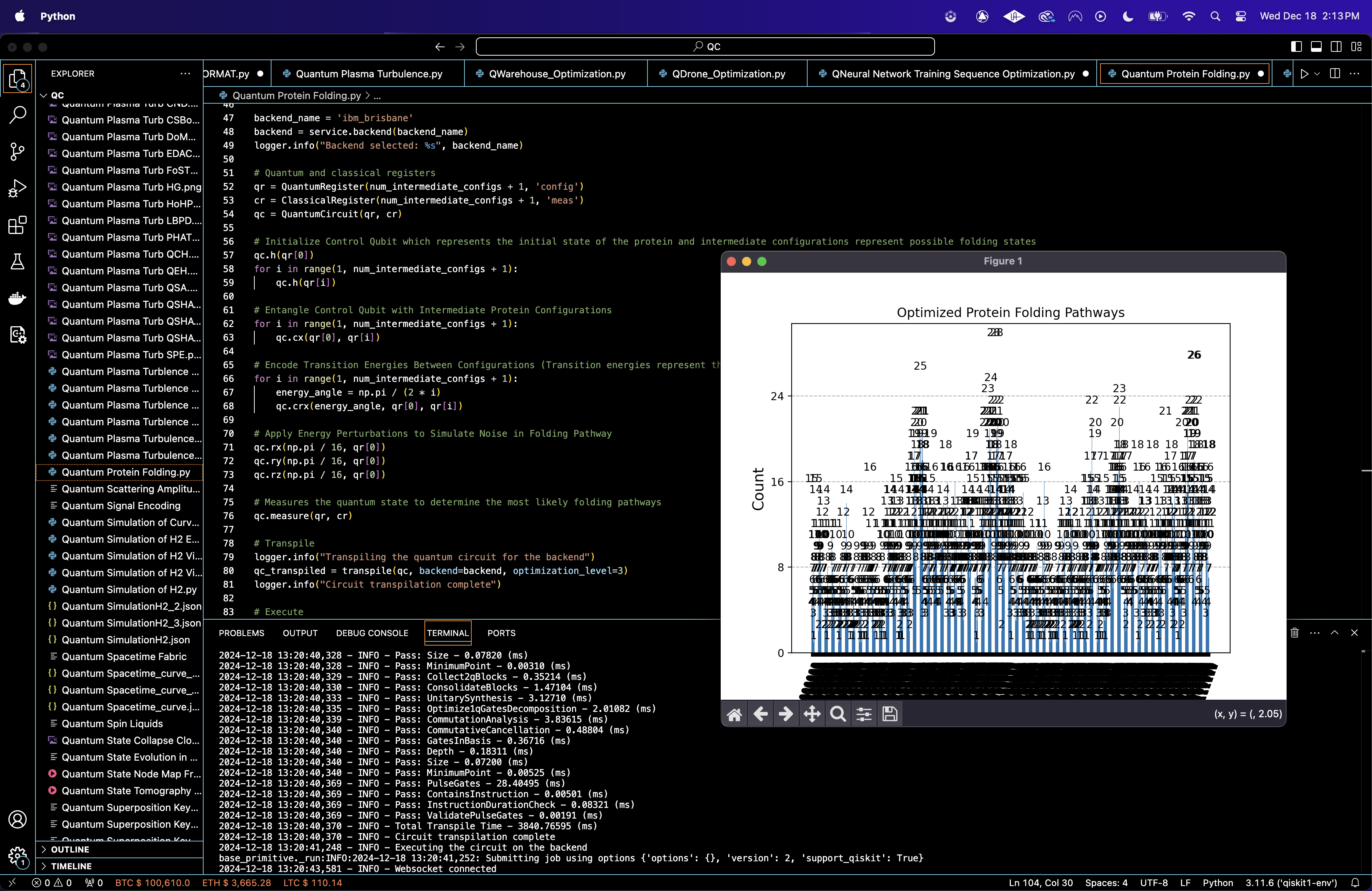
The quantum circuit is measured, with each bitstring representing a specific folding pathway. The frequency of each bitstring in the measurement results corresponds to the likelihood of that pathway being energetically favorable.
9. Transpilation
The circuit is transpiled for ibm_brisbane.
10. Results
The transpiled circuit is executed with 16,384 shots. Measurement results are extracted, and the counts for each bitstring are analyzed.
11. Visual
A histogram of the bitstring counts is plotted.
Top String: 01110100111 with 28 counts.
Top 10 Strings (by frequency):
01110100111 - 28 counts
01110100001 - 21 counts
01000110010 - 25 counts
01110011011 - 24 counts
11000110001 - 23 counts
01110001011 - 23 counts
01110111101 - 22 counts
11110110111 - 22 counts
11110100001 - 22 counts
11100011101 - 21 counts
These results confirm that specific folding pathways are energetically preferred, as indicated by their high recurrence.

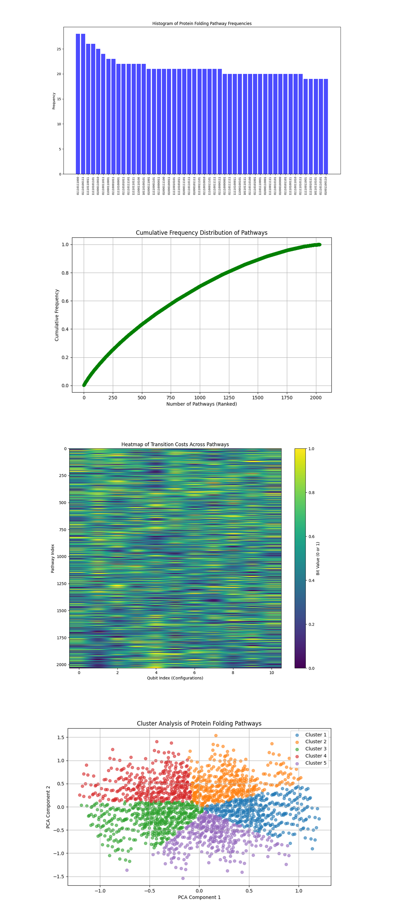
The Histogram of Protein Folding Pathway Frequencies above (code below) displays the frequencies of each bitstring (protein folding pathway) from the experiment, highlighting the most frequently measured pathways. Pathways with the highest frequencies represent the most energetically favorable folding states based on the quantum interference of the circuit. Dominant bitstrings indicate folding pathways with minimal free energy, aligning with the physical objective of protein folding. Lesser frequent bitstrings might reflect noise or energetically less favorable pathways.
The Cumulative Frequency Distribution of Pathways above (code below) shows the frequencies of pathways in ranked order to show how many pathways contribute to the majority of measurements. A steep initial rise in the cumulative frequency curve indicates that a small subset of pathways accounts for a large portion of the measurements. This aligns with the expected behavior that a few energetically favorable configurations dominate the folding process.
The Heatmap of Transition Costs Across Pathways above (code below) maps the bit values (0 or 1) for different pathways and qubits, effectively showing the structure of transitions between intermediate protein configurations. Clustering patterns or repetitive structures in the heatmap suggest symmetries in the folding process or recurring structural motifs in the protein. Areas with high contrast might represent configurations where energy differences between transitions are pronounced.
The Cluster Analysis of Protein Folding Pathways above (code below), using PCA and K-means clustering, plots groups pathways into clusters based on similarity in their bitstring representation. Distinct clusters represent families of folding pathways with shared structural or energetic properties. Clusters with higher density likely correspond to dominant folding patterns, while sparse clusters may reflect rare or suboptimal configurations.

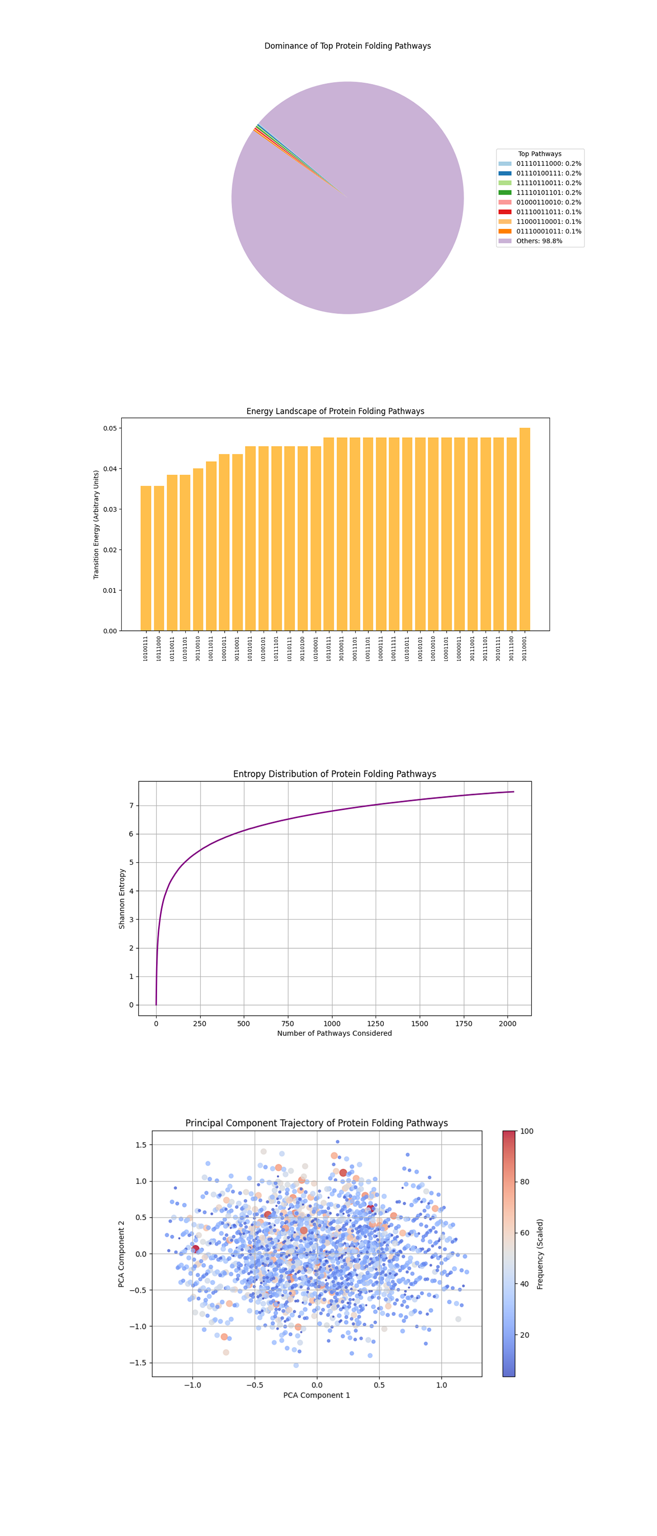
The Pathway Dominance Pie Chart chart above (code below) shows the proportion of measurement results contributed by the top pathways compared to others. 'Others' represents the sum of frequencies for all pathways outside the top contributors. The top pathways each contribute a small but significant percentage, indicating a long tail distribution where a few pathways dominate the remaining minority. The chart shows the quantum system’s ability to focus probability amplitudes on specific folding pathways.
The Energy Landscape Bar Plot above (code below) maps folding pathways (bitstrings) to their estimated transition energies. Lower transition energies represent more favorable pathways. The flat top clustering of energies at higher levels may indicate degeneracies or pathways that are energetically similar but less favorable. The lowest energy pathways are more likely to represent the protein’s folded state, minimizing free energy.
The Entropy Distribution above (code below) calculates the Shannon entropy as more pathways are included, showing how spread out or uncertain the measurements are across pathways. The steep initial rise in entropy indicates a diverse set of pathways contributing to the initial results. The curve eventually flattens, suggesting a saturation point where additional pathways contribute minimally to the overall uncertainty. High entropy in the early pathways reflects the inherent complexity and probabilistic nature of protein folding, while the saturation implies the quantum system’s focus on key pathways.
The Principal Component Trajectory of Pathways above (code below) reduces the high dimensional bitstring data into two components, grouping pathways by similarity. The size and color intensity of points correspond to their frequency. Dense clusters represent groups of pathways with similar folding properties, indicating common structural or energetic patterns. Outliers or sparsely distributed points may represent rare configurations that are less probable.

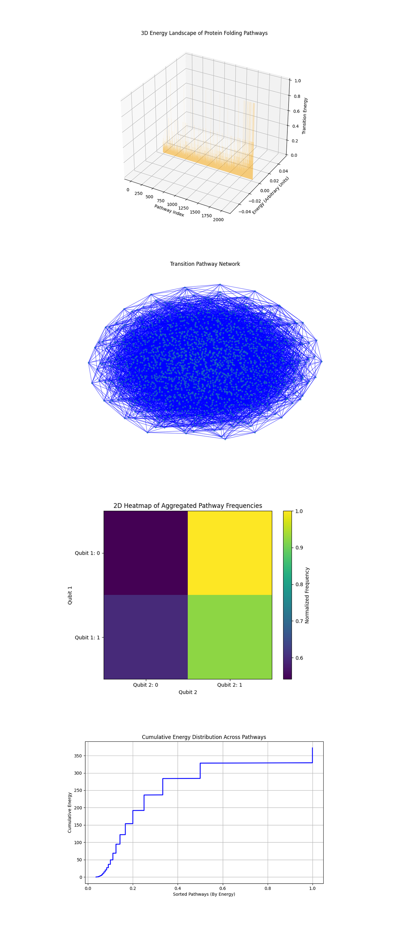
The 3D Energy Landscape of Protein Folding Pathways above (code below) shows the transition energy of pathways along their indices. The peaks and valleys represent different energy levels, showing how certain pathways dominate. High energy pathways are sparse, indicating a small number of configurations requiring significant computational effort. The clustering of lower energy pathways suggests that the majority of configurations are energetically favorable, reinforcing the idea that proteins naturally fold into low energy states.
The Transition Pathway Network above (code below) graphs where nodes represent pathways and the edges show possible transitions between them. The connectivity suggests that proteins can transition between multiple configurations before settling into their final folded state. The symmetry and density of the network highlight strength in the folding process, where multiple pathways may lead to similar final states.
The 2D Heatmap of Aggregated Pathway Frequencies above (code below) shows a grid based heatmap where the color intensity corresponds to the frequency of configurations associated with the first two qubits. Pathways starting with specific qubit states (Qubit 1: 0 and Qubit 2: 1) are more likely to be energetically favorable. The asymmetry in the heatmap suggests that certain initial conditions (qubit states) strongly influence the folding pathway's likelihood.
The Cumulative Energy Distribution Across Pathways above (code below) shows how the total energy accumulates as pathways are sorted by their energy. Most of the energy is concentrated in a small subset of pathways, aligning with the expectation that proteins fold through energetically efficient paths. The long tail of high energy states suggests that outlier configurations exist but contribute minimally.
In the end, this experiment explored protein folding optimization using IBM's 127-qubit quantum computer. The goal was to simulate folding pathways as quantum states, where each pathway represents a configuration of the protein, and the transitions between configurations correspond to the computational effort required to achieve minimal free energy. By encoding the folding landscape into quantum superpositions, entanglement, and rotations, the circuit used quantum interference to identify the most energetically favorable pathways.
Code:
# Imports
import numpy as np
import json
import pandas as pd
import logging
from qiskit import QuantumCircuit, QuantumRegister, ClassicalRegister, transpile
from qiskit_ibm_runtime import QiskitRuntimeService, Session, SamplerV2
from qiskit.visualization import plot_histogram
import matplotlib.pyplot as plt

# Logging
logging.basicConfig(level=logging. INFO, format='%(asctime)s - %(levelname)s - %(message)s')
logger = logging.getLogger(__name__)

# Load calibration data
def load_calibration_data(file_path):
    logger. info("Loading calibration data from %s", file_path)
    calibration_data = pd. read_csv(file_path)
    calibration_data.columns = calibration_data.columns.str.strip()
    logger. info("Calibration data loaded successfully")
    return calibration_data

# Parse calibration data
def select_best_qubits(calibration_data, n_qubits):
    logger. info("Selecting the best qubits based on T1, T2, and error rates")
    qubits_sorted = calibration_data.sort_values(by=['\u221ax (sx) error', 'T1 (us)', 'T2 (us)'], ascending=[True, False, False])
    best_qubits = qubits_sorted['Qubit'].head(n_qubits).tolist()
    logger. info("Selected qubits: %s", best_qubits)
    return best_qubits

# Load backend calibration data
calibration_file = '/Users/Downloads/ibm_brisbane_calibrations_2024-12-18T17_08_04Z.csv'
calibration_data = load_calibration_data(calibration_file)

# Select best qubits based on T1, T2, and error rates
num_intermediate_configs = 10
best_qubits = select_best_qubits(calibration_data, num_intermediate_configs + 1)

# IBMQ
logger. info("Setting up IBM Q service")
service = QiskitRuntimeService(
    channel='ibm_quantum',
    instance='ibm-q/open/main',
    token='YOUR_IBMQ_API_KEY_O-`'
)

backend_name = 'ibm_brisbane'
backend = service.backend(backend_name)
logger. info("Backend selected: %s", backend_name)

# Quantum and classical registers
qr = QuantumRegister(num_intermediate_configs + 1, 'config')
cr = ClassicalRegister(num_intermediate_configs + 1, 'meas')
qc = QuantumCircuit(qr, cr)

# Initialize Control Qubit which represents the initial state of the protein and intermediate configurations represent possible folding states
qc.h(qr[0])
for i in range(1, num_intermediate_configs + 1):
    qc.h(qr[i])

# Entangle Control Qubit with Intermediate Protein Configurations
for i in range(1, num_intermediate_configs + 1):
    qc. cx(qr[0], qr[i])

# Encode Transition Energies Between Configurations (Transition energies represent the free energy difference between folding states)
for i in range(1, num_intermediate_configs + 1):
    energy_angle = np.pi / (2 * i)
    qc.crx(energy_angle, qr[0], qr[i])

# Apply Energy Perturbations to Simulate Noise in Folding Pathway
qc.rx(np.pi / 16, qr[0])
qc.ry(np.pi / 16, qr[0])
qc.rz(np.pi / 16, qr[0])

# Measures the most likely folding pathways
qc.measure(qr, cr)

# Transpile
logger. info("Transpiling the quantum circuit for the backend")
qc_transpiled = transpile(qc, backend=backend, optimization_level=3)
logger. info("Circuit transpilation complete")

# Execute
shots = 16384
with Session(service=service, backend=backend) as session:
    sampler = SamplerV2(session=session)
    logger. info("Executing the circuit on the backend")
    job = sampler. run([qc_transpiled], shots=shots)
    job_result = job.result()

    # Extract BitArray counts
    data_bin = job_result._pub_results[0]['__value__']['data']
    bit_array = data_bin['meas']  # Extract the BitArray
    counts = bit_array.get_counts()  # Use get_counts method

    # Save json
    results_data = {"raw_counts": counts}
    file_path = '/Users/Documents/QProtein_Folding_Results_0.json'
    with open(file_path, 'w') as f:
        json.dump(results_data, f, indent=4)
    logger. info("Results saved to %s", file_path)

# Visualizes the likelihood of each folding pathway
plot_histogram(counts)
plt.title("Optimized Protein Folding Pathways")
plt. show()

Code For All Visuals From Run Data
# Imports
import matplotlib.pyplot as plt
from collections import Counter
import numpy as np
import json
from scipy.stats import entropy
from sklearn.decomposition import PCA
from mpl_toolkits.mplot3d import Axes3D
import networkx as nx
from scipy.stats import gaussian_kde

# Load results
file_path = '/Users/Documents/QProtein_Folding_Results_0.json'
with open(file_path, 'r') as f:
    data = json.load(f)

raw_counts = data['raw_counts']

# Histogram of Bitstring Frequencies
def plot_histogram(raw_counts):
    sorted_counts = sorted(raw_counts.items(), key=lambda x: x[1], reverse=True)
    bitstrings, frequencies = zip(*sorted_counts[:50])
    plt.figure(figsize=(15, 8))
    plt. bar(bitstrings, frequencies, color='blue', alpha=0.7)
    plt.xticks(rotation=90, fontsize=8)
    plt.xlabel("Bitstrings (Protein Folding Pathways)")
    plt.ylabel("Frequency")
    plt.title("Histogram of Protein Folding Pathway Frequencies")
    plt. show()

# Cumulative Frequency Distribution
def plot_cumulative_frequency(raw_counts):
    sorted_frequencies = sorted(raw_counts.values(), reverse=True)
    cumulative = np.cumsum(sorted_frequencies) / sum(sorted_frequencies)
    plt.figure(figsize=(10, 6))
    plt.plot(cumulative, marker='o', linestyle='-', color='green')
    plt.xlabel("Number of Pathways (Ranked)")
    plt.ylabel("Cumulative Frequency")
    plt.title("Cumulative Frequency Distribution of Pathways")
    plt.grid(True)
    plt. show()

# Heatmap of Transition Costs
def plot_heatmap(raw_counts):
    pathway_matrix = []
    for bitstring, frequency in raw_counts.items():
        pathway_matrix.append([int(bit) for bit in bitstring])
    pathway_matrix = np.array(pathway_matrix)
    plt.figure(figsize=(12, 10))
    plt.imshow(pathway_matrix, aspect='auto', cmap='viridis')
    plt.colorbar(label="Bit Value (0 or 1)")
    plt.xlabel("Qubit Index (Configurations)")
    plt.ylabel("Pathway Index")
    plt.title("Heatmap of Transition Costs Across Pathways")
    plt. show()

# Cluster Analysis of Pathways
from sklearn.decomposition import PCA
from sklearn.cluster import KMeans

def plot_cluster_analysis(raw_counts):
    pathway_matrix = np.array([[int(bit) for bit in bitstring] for bitstring in raw_counts.keys()])
    pca = PCA(n_components=2)
    reduced_data = pca. fit_transform(pathway_matrix)
    kmeans = KMeans(n_clusters=5).fit(reduced_data)
    labels = kmeans.labels_

    plt.figure(figsize=(10, 6))
    for i in range(5):
        cluster_data = reduced_data[labels == i]
        plt.scatter(cluster_data[:, 0], cluster_data[:, 1], label=f'Cluster {i+1}', alpha=0.6)
    plt.xlabel("PCA Component 1")
    plt.ylabel("PCA Component 2")
    plt.title("Cluster Analysis of Protein Folding Pathways")
    plt.legend()
    plt.grid(True)
    plt. show()

# Call
plot_histogram(raw_counts)
plot_cumulative_frequency(raw_counts)
plot_heatmap(raw_counts)
plot_cluster_analysis(raw_counts)

# Pathway Dominance Pie Chart
def plot_pathway_dominance_pie(raw_counts):
    top_paths = Counter(raw_counts).most_common(8)
    labels, values = zip(*top_paths)
    other_sum = sum(raw_counts.values()) - sum(values)
    labels = list(labels) + ["Others"]
    values = list(values) + [other_sum]

    # Calculate percentages
    total = sum(values)
    percentages = [f"{(value / total) * 100:.1f}%" for value in values]

    plt.figure(figsize=(10, 8))
    wedges = plt.pie(
        values, labels=None, startangle=140, colors=plt. cm.Paired.colors
    )[0]

    # Add legend
    legend_labels = [f"{label}: {percent}" for label, percent in zip(labels, percentages)]
    plt.legend(wedges, legend_labels, title="Top Pathways", loc="center left", bbox_to_anchor=(1, 0.5))
    plt.title("Dominance of Top Protein Folding Pathways")
    plt. show()

# Energy Landscape Bar Plot
def plot_energy_landscape(raw_counts):
    bitstrings = list(raw_counts.keys())
    frequencies = list(raw_counts.values())

    energies = [1 / freq if freq > 0 else 0 for freq in frequencies]
    sorted_indices = np.argsort(energies)
    sorted_energies = np.array(energies)[sorted_indices]
    sorted_bitstrings = np.array(bitstrings)[sorted_indices]

    plt.figure(figsize=(12, 6))
    plt. bar(sorted_bitstrings[:30], sorted_energies[:30], color='orange', alpha=0.7)
    plt.xticks(rotation=90, fontsize=8)
    plt.xlabel("Bitstrings (Protein Folding Pathways)")
    plt.ylabel("Transition Energy (Arbitrary Units)")
    plt.title("Energy Landscape of Protein Folding Pathways")
    plt. show()

# Entropy Distribution
def plot_entropy_distribution(raw_counts):
    frequencies = list(raw_counts.values())
    total = sum(frequencies)
    probabilities = [freq / total for freq in frequencies]
    entropy_values = [entropy(probabilities[:k]) for k in range(1, len(probabilities) + 1)]

    plt.figure(figsize=(10, 6))
    plt.plot(range(1, len(probabilities) + 1), entropy_values, color='purple', linewidth=2)
    plt.xlabel("Number of Pathways Considered")
    plt.ylabel("Shannon Entropy")
    plt.title("Entropy Distribution of Protein Folding Pathways")
    plt.grid(True)
    plt. show()

# Principal Component Trajectory
def plot_pca_trajectory(raw_counts):
    pathway_matrix = np.array([[int(bit) for bit in bitstring] for bitstring in raw_counts.keys()])
    pca = PCA(n_components=2)
    reduced_data = pca. fit_transform(pathway_matrix)
    frequencies = np.array(list(raw_counts.values()))
    sizes = frequencies / frequencies.max() * 100

    plt.figure(figsize=(10, 6))
    plt.scatter(reduced_data[:, 0], reduced_data[:, 1], s=sizes, c=sizes, cmap='coolwarm', alpha=0.8)
    plt.colorbar(label="Frequency (Scaled)")
    plt.xlabel("PCA Component 1")
    plt.ylabel("PCA Component 2")
    plt.title("Principal Component Trajectory of Protein Folding Pathways")
    plt.grid(True)
    plt. show()

# Call
plot_pathway_dominance_pie(raw_counts)
plot_energy_landscape(raw_counts)
plot_entropy_distribution(raw_counts)
plot_pca_trajectory(raw_counts)

# 3D Energy Landscape
def plot_3d_energy_landscape(raw_counts):
    bitstrings = list(raw_counts.keys())
    frequencies = list(raw_counts.values())

    energies = [1 / freq if freq > 0 else 0 for freq in frequencies]
    indices = range(len(bitstrings))

    fig = plt.figure(figsize=(10, 8))
    ax = fig.add_subplot(111, projection='3d')
    ax. bar(indices, energies, zs=0, zdir='y', alpha=0.8, color='orange')

    ax.set_xlabel("Pathway Index")
    ax.set_ylabel("Energy (Arbitrary Units)")
    ax.set_zlabel("Transition Energy")
    ax.set_title("3D Energy Landscape of Protein Folding Pathways")
    plt. show()

# Transition Pathway Network
def plot_transition_pathway_network(raw_counts):
    bitstrings = list(raw_counts.keys())
    G = nx.Graph()

    for i, bs1 in enumerate(bitstrings):
        for j, bs2 in enumerate(bitstrings):
            if i < j and sum(c1 != c2 for c1, c2 in zip(bs1, bs2)) == 1:
                G.add_edge(bs1, bs2)

    plt.figure(figsize=(12, 8))
    plt.title("Transition Pathway Network")
    pos = nx.spring_layout(G, seed=42)
    nx.draw(G, pos, with_labels=False, node_size=10, edge_color="blue", alpha=0.6)
    plt. show()

# Probability Density Heatmap
def plot_2d_heatmap_pathways(raw_counts):
    # Convert pathways to matrix form
    pathway_matrix = np.array([[int(bit) for bit in bitstring] for bitstring in raw_counts.keys()])
    frequencies = np.array(list(raw_counts.values()))

    grid_size = (2, 2)
    heatmap = np.zeros(grid_size, dtype=float)

    for bits, freq in zip(pathway_matrix, frequencies):
        if len(bits) >= 2:
            row, col = bits[:2]
            heatmap[row, col] += freq

    # Normalize the heatmap
    heatmap /= heatmap.max()

    # Plot the 2D heatmap
    plt.figure(figsize=(8, 6))
    plt.imshow(heatmap, cmap="viridis", interpolation="nearest")
    plt.colorbar(label="Normalized Frequency")
    plt.xticks(ticks=[0, 1], labels=["Qubit 2: 0", "Qubit 2: 1"])
    plt.yticks(ticks=[0, 1], labels=["Qubit 1: 0", "Qubit 1: 1"])
    plt.xlabel("Qubit 2")
    plt.ylabel("Qubit 1")
    plt.title("2D Heatmap of Aggregated Pathway Frequencies")
    plt. show()

# Energy Distribution Curve
def plot_cumulative_energy_distribution(raw_counts):
    # Extract frequencies and compute energies
    frequencies = np.array(list(raw_counts.values()))
    energies = np.array([1 / freq if freq > 0 else 0 for freq in frequencies])  # Energy inversely proportional to frequency

    # Sort energies in ascending order
    sorted_energies = np.sort(energies)

    # Compute cumulative energy
    cumulative_energy = np.cumsum(sorted_energies)

    # Plot the cumulative energy distribution
    plt.figure(figsize=(10, 6))
    plt.plot(sorted_energies, cumulative_energy, color='blue', linewidth=2)
    plt.xlabel("Sorted Pathways (By Energy)")
    plt.ylabel("Cumulative Energy")
    plt.title("Cumulative Energy Distribution Across Pathways")
    plt.grid(True)
    plt. show()

# Call
plot_3d_energy_landscape(raw_counts)
plot_transition_pathway_network(raw_counts)
plot_2d_heatmap_pathways(raw_counts)
plot_cumulative_energy_distribution(raw_counts)

# End
