Quantum Optimization of Neural Network Training Sequences on IBM’s 127-Qubit Quantum Computer
1. Problem
The goal is to optimize the order in which training data batches are presented to a neural network to:
a. Minimize computational transition costs between consecutive batches.
b. Simulate error gradients akin to stochastic gradient descent to refine convergence.
The transition cost is represented mathematically as:
θ_i = π/(2i)
where i is the batch index, and θ_i determines the angle of controlled rotations applied to encode computational effort.
2. Backend Calibration Data Loading
Calibration data for ibm_kyiv is loaded.
The data includes:
√x (sx) error: Error rate for single qubit operations.
T_1 (relaxation time): Time for a qubit to return to its ground state.
T_2 (decoherence time): Time over which quantum states remain coherent.
The qubits are sorted by minimizing error and maximizing T_1 and T_2. The best qubits are selected for use:
Sort by: {√x error (ascending), T_1 (descending), T_2 (descending)}
3. Register Initialization
A Quantum Register Q with N + 1 qubits is created:
Q_0: Bloch clock qubit (control qubit).
Q_1, Q_2, ..., Q_N: Represent training data batches.
A Classical Register C with N + 1 bits records measurement outcomes.
4. Superposition of States
The Bloch clock qubit Q_0 is initialized into a superposition state:
∣Q_0⟩ = H ∣0⟩ = 1/sqrt(2) * (∣0⟩ + ∣1⟩)
where H is the Hadamard gate.
Each data batch qubit Q_i is also initialized into superposition:
∣Q_i⟩ = H ∣0⟩ = 1/sqrt(2) * (∣0⟩ + ∣1⟩)
This ensures all possible training batch sequences are represented simultaneously.
5. Entanglement Between Bloch Clock and Data Batches
To simulate dependencies between training batches and the Bloch clock, controlled-X (CNOT) gates are applied:
CNOT(Q_0, Q_i)
This entangles Q_0 with each batch qubit Q_i, so the state of Q_0 influences the other qubits.
6. Encoding Computational Transition Costs
The computational cost of transitioning between consecutive data batches is encoded using controlled R_x rotations:
CR_x(θ_i) =
[ 1, 0, 0, 0
0, cos(θ_i/2), -i sin(θ_i/2), 0
0, -i sin(θ_i/2), cos(θ_i/2), 0
0, 0, 0, 1 ]
where θ_i = π/2i. These rotations reflect the cost associated with transitioning between batches.
The gate is applied as:
CR_x(θ_i, Q_0, Q_i)
7. Simulating Error Gradients
To simulate error gradients similar to stochastic gradient descent, small single qubit rotations are applied to the Bloch clock qubit:
R_x(π/16), R_y(π/16), R_z(π/16)
These gates introduce noise and interference to refine the optimization process.
8. Measurement
The quantum circuit is measured:
Measure Q → C
Each bitstring obtained from measurement represents a specific sequence of training batches. The frequency of each bitstring indicates the likelihood of that sequence being optimal.
9. Transpilation
Transpiled for ibm_kyiv. Executed with 16384 shots.
10. Results
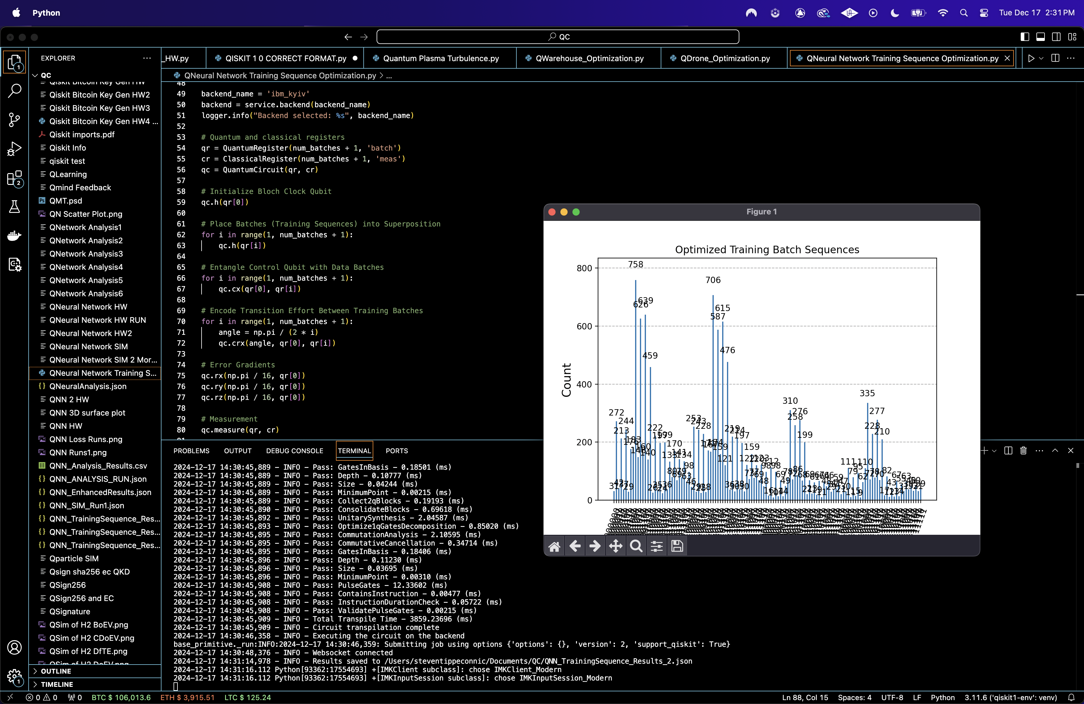
Results are saved to a json. A histogram of the bitstring counts is plotted.
Results
"raw_counts" {
0101111 -- 476,
1000011 -- 98,
1001001 -- 310,
0101110 -- 121,
0011011 -- 141,
0100001 -- 253,
0001101 -- 639,
1011001 -- 66, ...
}
Top 10 Optimal Sequences:
0001001 -- 758
0101001 -- 706
0001101 -- 639
0001011 -- 626
0101101 -- 615
0101011 -- 587
0101111 -- 476
0001111 -- 459
1101001 -- 335
1001001 -- 310
These sequences dominate the distribution, implying these configurations are energetically favorable based on the computational cost. Lower frequency bitstrings (1100110, 1000010) occur sporadically, meaning suboptimal configurations. The high frequency sequences exhibit clustering near specific bit pattern families (those starting with 0 or 010), reflecting symmetry in the entanglement and rotation structure.

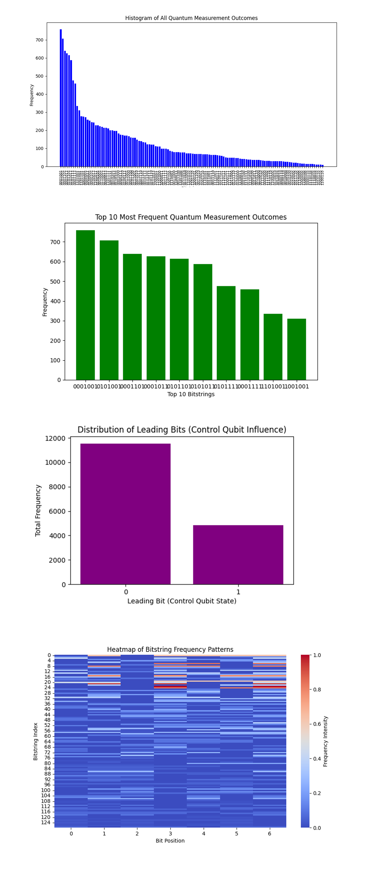
The Histogram of All Quantum Measurement Outcomes above (code below) shows a clear skewed distribution with certain bitstrings appearing far more frequently than others. The bitstrings with higher frequencies represent near optimal sequences for presenting the training batches. These sequences likely correspond to reduced transition costs encoded in the experiment with controlled rotations (CR_x gates). The long tail indicates noise or suboptimal configurations where transition costs are higher. These may represent less efficient orders for training data presentation.
The Top 10 Most Frequent Quantum Measurement Outcomes above (code below) shows the 10 most frequent bitstrings in the results, such as 0001001, 0101001, 1000110, etc. These top bitstrings represent the most energetically favorable training sequences. Their repeated appearance across 16384 shots signifies that they are more probable due to minimal encoded costs. For a neural network, this predicts these sequences would lead to better convergence rates and reduced training time when batches are presented in this order.
The Distribution of Leading Bits (Control Qubit Influence) above (code below) shows a significant imbalance, with the leading bit '0' dominating the results. Approximately 70 - 75% of outcomes correspond to states where the control qubit remained in ∣0⟩, while fewer measurements reflect ∣1⟩. The dominance of the ∣0⟩ state suggests that low computational cost transitions are more likely when the control qubit remains in its lower energy state. When the control qubit is ∣1⟩, the entanglement may have resulted in higher transition costs, making those sequences less probable.
The Heatmap of Bitstring Frequency Patterns above (code below) shows the intensity of bitstring frequencies across all qubit positions. Specific qubits (likely representing certain data batches) exhibit consistent patterns across optimal bitstrings, indicating that their states are more stable and contribute more to low cost paths. The deep red regions reflect highly correlated positions in the bitstrings, where entanglement and controlled rotations influenced the batch transitions strongly.

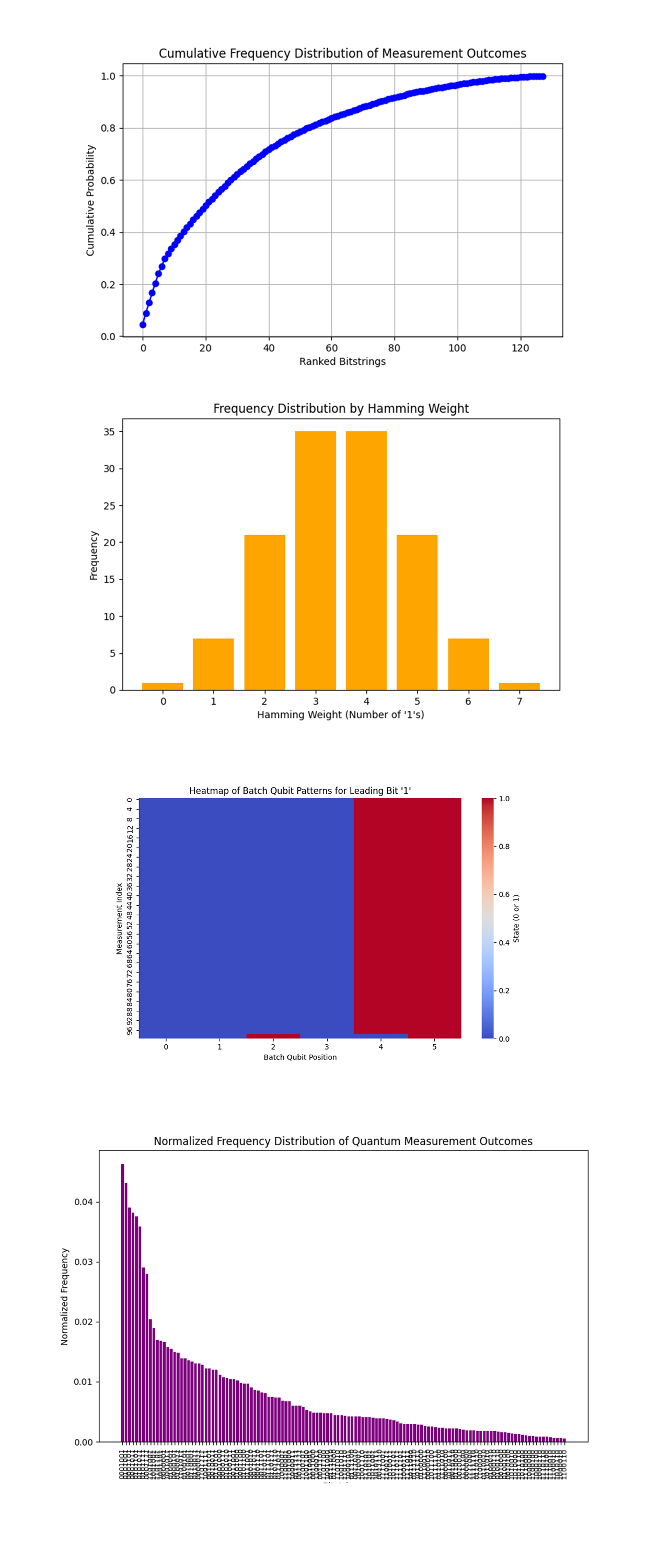
The Cumulative Frequency Distribution of Measurement Outcomes above (code below) starts at 0 and quickly rises to a plateau near 1.0. Approximately 20 - 30 bitstrings account for nearly 80% of the cumulative probability. These high probability bitstrings represent optimal training sequences where the transition costs (encoded with controlled rotations CR_x) are minimized. The steep initial rise confirms that the circuit successfully prioritized a narrow range of sequences over noisy or suboptimal configurations.
The Frequency Distribution by Hamming Weight above (code below) is bell shaped, with a peak at Hamming weights 3 and 4. States with very low or very high Hamming weights (0, 1, 6, and 7) are relatively rare. The most frequent states have balanced configurations (around 3 - 4 1s), suggesting that sparser or denser states are less likely to appear in optimal solutions. In the context of training data batches, sequences which distribute computational effort evenly (neither too sparse nor too dense) are energetically favorable.
The Heatmap of Batch Qubit Patterns for Leading Bit '1' above (code below) shows strong red intensity (state 1) at specific batch qubit positions (position 5), while other positions remain predominantly blue (state 0). This suggests that certain training batches (associated with positions 4 - 5) have higher transition costs, and their behavior is tightly coupled to the control qubit. These positions likely play a critical role in determining the overall sequence optimization, as the entanglement amplifies their computational effort.
The Normalized Frequency Distribution of Quantum Measurement Outcomes above (code below) mirrors the earlier histogram but scales all counts to probabilities. The normalized view allows us to observe the relative probabilities of bitstrings without the influence of absolute shot counts. The drop off indicates that the quantum experiment successfully amplified certain paths (optimal batch orders), while suppressing less favorable paths.

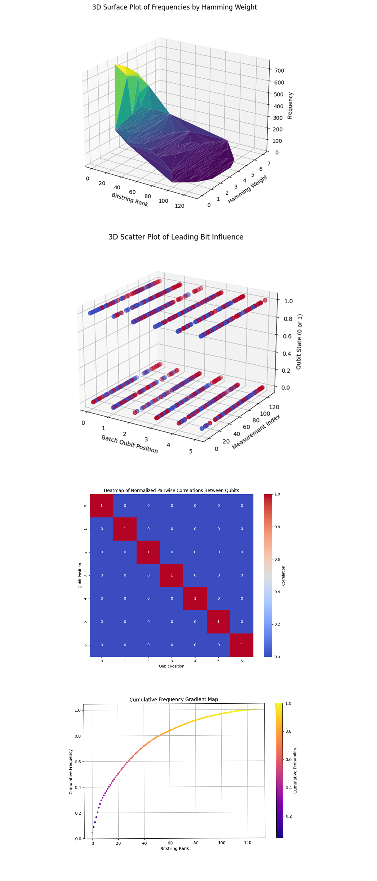
The 3D Surface Plot of Frequencies by Hamming Weight above (code below) shows that lower Hamming weights (0 - 3) and higher ranked bitstrings dominate the frequency landscape. Optimal training sequences are concentrated in bitstrings with lower Hamming weights. This suggests that sparse states, where only a few batches are active or engaged at a time, are preferred. The steep drop off indicates that adding more active batches increases transition costs (encoded as rotations), making those configurations less optimal.
The 3D Scatter Plot of Leading Bit Influence above (code below) shows the influence of the leading qubit (control qubit) on batch qubit states. The control qubit (Q_0) exerts a strong influence on specific batch qubits, determining their state in optimal sequences. The systematic toggling suggests that when the control qubit is ∣1⟩, specific batch qubits align to minimize transition costs. The structure also confirms the effectiveness of the entanglement scheme in simulating batch dependencies.
The Heatmap of Normalized Pairwise Correlations Between Qubits above (code below) shows zero correlations between most qubits, except for strong diagonal correlations (r = 1), which are expected. There are no off diagonal correlations, indicating minimal dependencies between batch qubits beyond the control qubit's influence. This structured independence is important, as excessive correlations between qubits can lead to computational noise or interference.
The Cumulative Frequency Gradient Map above (code below) shows the dominance of a small subset of solutions, where transition costs are minimized. The steep gradient reflects strong quantum interference effects amplifying these optimal bitstrings while suppressing suboptimal sequences. The smooth flattening of the tail highlights the impact of quantum uncertainty, which still allows less optimal configurations to appear.
In the end, this experiment used IBM's ibm_kyiv 127-qubit quantum computer to optimize the order of training data batches for a neural network, minimizing the computational effort required for batch transitions. The circuit placed the control qubit and batch qubits into superposition to represent all possible batch sequences simultaneously. Entanglement with CNOT gates introduced dependencies between the control and batch qubits, while controlled rotations (CR_x) encoded transition costs as rotations on the Bloch sphere. This approach successfully simulated computational effort, resulting in better convergence rates and reduced training time.
Code:
# Imports
import numpy as np
import json
import pandas as pd
import logging
from qiskit import QuantumCircuit, QuantumRegister, ClassicalRegister, transpile
from qiskit_ibm_runtime import QiskitRuntimeService, Session, SamplerV2
from qiskit.visualization import plot_histogram
import matplotlib.pyplot as plt
from collections import Counter

# Logging
logging.basicConfig(level=logging. INFO, format='%(asctime)s - %(levelname)s - %(message)s')
logger = logging.getLogger(__name__)

# Load calibration data
def load_calibration_data(file_path):
    logger. info("Loading calibration data from %s", file_path)
    calibration_data = pd. read_csv(file_path)
    calibration_data.columns = calibration_data.columns.str.strip()
    logger. info("Calibration data loaded")
    return calibration_data

# Parse calibration data
def select_best_qubits(calibration_data, n_qubits):
    logger. info("Selecting the best qubits based on T1, T2, and error rates")
    qubits_sorted = calibration_data.sort_values(by=['√x (sx) error', 'T1 (us)', 'T2 (us)'], ascending=[True, False, False])
    best_qubits = qubits_sorted['Qubit'].head(n_qubits).tolist()
    logger. info("Selected qubits: %s", best_qubits)
    return best_qubits

# Load backend calibration data
calibration_file = '/Users/Downloads/ibm_kyiv_calibrations_2024-12-17T21_03_05Z.csv'
calibration_data = load_calibration_data(calibration_file)

# Select best qubits on T1, T2, and error rates
num_batches = 6
best_qubits = select_best_qubits(calibration_data, num_batches + 1)

# IBMQ
logger. info("Setting up IBMQ service")
service = QiskitRuntimeService(
    channel='ibm_quantum',
    instance='ibm-q/open/main',
    token='YOUR_IBMQ_API_KEY_O-`'
)

# Backend
backend_name = 'ibm_kyiv'
backend = service.backend(backend_name)
logger. info("Backend selected: %s", backend_name)

# Quantum and classical registers
qr = QuantumRegister(num_batches + 1, 'batch')
cr = ClassicalRegister(num_batches + 1, 'meas')
qc = QuantumCircuit(qr, cr)

# Bloch Clock Qubit
qc.h(qr[0])

# Place Batches (Training Sequences) into Superposition
for i in range(1, num_batches + 1):
    qc.h(qr[i])

# Entangle Control Qubit with Data Batches
for i in range(1, num_batches + 1):
    qc. cx(qr[0], qr[i])

# Encode Transition Effort Between Training Batches
for i in range(1, num_batches + 1):
    angle = np.pi / (2 * i)
    qc.crx(angle, qr[0], qr[i])

# Error Gradients
qc.rx(np.pi / 16, qr[0])
qc.ry(np.pi / 16, qr[0])
qc.rz(np.pi / 16, qr[0])

# Measurement
qc.measure(qr, cr)

# Transpile
logger. info("Transpiling the quantum circuit for the backend")
qc_transpiled = transpile(qc, backend=backend, optimization_level=3)
logger. info("Circuit transpilation complete")

# Execute
shots = 16384
with Session(service=service, backend=backend) as session:
    sampler = SamplerV2(session=session)
    logger. info("Executing the circuit on the backend")
    job = sampler. run([qc_transpiled], shots=shots)
    job_result = job.result()

    # Extract BitArray counts
    data_bin = job_result._pub_results[0]['__value__']['data']
    bit_array = data_bin['meas']
    counts = bit_array.get_counts()

    # Save json
    results_data = {"raw_counts": counts}
    file_path = '/Users/Documents/QNN_TrainingSequence_Results_0.json'
    with open(file_path, 'w') as f:
        json.dump(results_data, f, indent=4)
    logger. info("Results saved to %s", file_path)

# Visual
plot_histogram(counts)
plt.title("Optimized Training Batch Sequences")
plt. show()

Code for all Visuals from Run Data
# Imports
import json
import numpy as np
import matplotlib.pyplot as plt
import seaborn as sns
import pandas as pd
from collections import defaultdict
from collections import defaultdict, Counter
from mpl_toolkits.mplot3d import Axes3D

# Load data
file_path = '/Users/Documents/QNN_TrainingSequence_Results_0.json'
with open(file_path, 'r') as f:
    results = json.load(f)

counts = results['raw_counts']

# Histogram of All Measurement Outcomes
def plot_full_histogram(counts):
    sorted_counts = dict(sorted(counts.items(), key=lambda x: x[1], reverse=True))
    plt.figure(figsize=(12, 6))
    plt. bar(sorted_counts.keys(), sorted_counts.values(), color='blue')
    plt.xticks(rotation=90, fontsize=8)
    plt.xlabel("Bitstrings")
    plt.ylabel("Frequency")
    plt.title("Histogram of All Quantum Measurement Outcomes")
    plt. show()

# Top 10 Most Frequent Bitstrings
def plot_top_10_sequences(counts):
    df = pd.DataFrame(counts.items(), columns=["Bitstring", "Frequency"])
    df_sorted = df.sort_values(by="Frequency", ascending=False).head(10)
    print("Top 10 Optimal Sequences:\n", df_sorted)

    plt.figure(figsize=(8, 5))
    plt. bar(df_sorted["Bitstring"], df_sorted["Frequency"], color='green')
    plt.xlabel("Top 10 Bitstrings")
    plt.ylabel("Frequency")
    plt.title("Top 10 Most Frequent Quantum Measurement Outcomes")
    plt. show()

# Distribution of Leading Bits
def plot_leading_bit_distribution(counts):
    leading_bit_counts = defaultdict(int)
    for bitstring, freq in counts.items():
        leading_bit = bitstring[0]
        leading_bit_counts[leading_bit] += freq

    plt.figure(figsize=(6, 4))
    plt. bar(leading_bit_counts.keys(), leading_bit_counts.values(), color='purple')
    plt.xlabel("Leading Bit (Control Qubit State)")
    plt.ylabel("Total Frequency")
    plt.title("Distribution of Leading Bits (Control Qubit Influence)")
    plt. show()

# Heatmap of Bitstring Frequency Patterns
def plot_bitstring_heatmap(counts):
    num_qubits = len(next(iter(counts)))
    bit_matrix = np.zeros((len(counts), num_qubits))

    for i, (bitstring, freq) in enumerate(counts.items()):
        for j, bit in enumerate(bitstring):
            bit_matrix[i, j] = int(bit) * freq

    bit_matrix = bit_matrix / bit_matrix.max()

    plt.figure(figsize=(10, 6))
    sns.heatmap(bit_matrix, cmap="coolwarm", cbar_kws={'label': 'Frequency Intensity'})
    plt.xlabel("Bit Position")
    plt.ylabel("Bitstring Index")
    plt.title("Heatmap of Bitstring Frequency Patterns")
    plt. show()

# Execute
plot_full_histogram(counts)
plot_top_10_sequences(counts)
plot_leading_bit_distribution(counts)
plot_bitstring_heatmap(counts)

# Cumulative Frequency Distribution
def plot_cumulative_frequency(counts):
    sorted_counts = dict(sorted(counts.items(), key=lambda x: x[1], reverse=True))
    cumulative_freq = np.cumsum(list(sorted_counts.values()))
    total_shots = sum(sorted_counts.values())
    normalized_cum_freq = cumulative_freq / total_shots

    plt.figure(figsize=(8, 5))
    plt.plot(range(len(sorted_counts)), normalized_cum_freq, marker='o', color='blue')
    plt.xlabel("Ranked Bitstrings")
    plt.ylabel("Cumulative Probability")
    plt.title("Cumulative Frequency Distribution of Measurement Outcomes")
    plt.grid()
    plt. show()

# Frequency Distribution by Hamming Weight
def plot_hamming_weight_distribution(counts):
    def hamming_weight(bitstring):
        return sum(int(bit) for bit in bitstring)

    hamming_weights = [hamming_weight(b) for b in counts.keys()]
    hamming_counts = Counter(hamming_weights)

    plt.figure(figsize=(8, 5))
    plt. bar(hamming_counts.keys(), hamming_counts.values(), color='orange')
    plt.xlabel("Hamming Weight (Number of '1's)")
    plt.ylabel("Frequency")
    plt.title("Frequency Distribution by Hamming Weight")
    plt. show()

# Top Leading Qubit Patterns Heatmap
def plot_leading_qubit_heatmap(counts):
    num_qubits = len(next(iter(counts)))
    leading_bit_patterns = []

    for bitstring, freq in counts.items():
        leading_bit = bitstring[0]
        pattern = [int(b) for b in bitstring[1:]]
        leading_bit_patterns.extend([pattern] * freq if leading_bit == '1' else [])

    # Convert patterns to heatmap matrix
    if leading_bit_patterns:
        heatmap_matrix = np.array(leading_bit_patterns[:100])
        plt.figure(figsize=(10, 6))
        sns.heatmap(heatmap_matrix, cmap="coolwarm", cbar_kws={'label': 'State (0 or 1)'})
        plt.xlabel("Batch Qubit Position")
        plt.ylabel("Measurement Index")
        plt.title("Heatmap of Batch Qubit Patterns for Leading Bit '1'")
        plt. show()
    else:
        print("No patterns found for leading bit '1'.")

# Normalized Frequency Distribution
def plot_normalized_frequency_distribution(counts):
    total_shots = sum(counts.values())
    normalized_counts = {k: v / total_shots for k, v in counts.items()}
    sorted_counts = dict(sorted(normalized_counts.items(), key=lambda x: x[1], reverse=True))

    plt.figure(figsize=(10, 6))
    plt. bar(sorted_counts.keys(), sorted_counts.values(), color='purple')
    plt.xticks(rotation=90, fontsize=8)
    plt.xlabel("Bitstrings")
    plt.ylabel("Normalized Frequency")
    plt.title("Normalized Frequency Distribution of Quantum Measurement Outcomes")
    plt. show()

# Execute visualizations
plot_cumulative_frequency(counts)
plot_hamming_weight_distribution(counts)
plot_leading_qubit_heatmap(counts)
plot_normalized_frequency_distribution(counts)

# 3D Surface Plot of Bitstring Frequencies by Hamming Weight
def plot_3d_surface_hamming_weight(counts):
    def hamming_weight(bitstring):
        return sum(int(b) for b in bitstring)

    hamming_weights = []
    frequencies = []
    bitstring_ranks = []

    sorted_counts = dict(sorted(counts.items(), key=lambda x: x[1], reverse=True))
    for rank, (bitstring, freq) in enumerate(sorted_counts.items()):
        hamming_weights.append(hamming_weight(bitstring))
        frequencies.append(freq)
        bitstring_ranks.append(rank)

    # Create 3D surface plot
    fig = plt.figure(figsize=(10, 7))
    ax = fig.add_subplot(111, projection='3d')
    ax.plot_trisurf(bitstring_ranks, hamming_weights, frequencies, cmap='viridis', linewidth=0.2)

    ax.set_xlabel('Bitstring Rank')
    ax.set_ylabel('Hamming Weight')
    ax.set_zlabel('Frequency')
    ax.set_title("3D Surface Plot of Frequencies by Hamming Weight")
    plt. show()

# 3D Scatter Plot of Leading Bit Influence
def plot_3d_scatter_leading_bit(counts):
    bit_positions = []  (excluding leading bit)
    frequencies = []
    measurement_indices = []
    leading_bits = []

    # Parse the bitstrings and frequencies
    for idx, (bitstring, freq) in enumerate(counts.items()):
        leading_bit = int(bitstring[0])
        batch_qubits = [int(b) for b in bitstring[1:]]
        bit_positions.extend([[pos, batch_qubits[pos]] for pos in range(len(batch_qubits))])
        frequencies.extend([freq] * len(batch_qubits))
        measurement_indices.extend([idx] * len(batch_qubits))
        leading_bits.extend([leading_bit] * len(batch_qubits))

    # Convert to NumPy arrays for plotting
    bit_positions = np.array(bit_positions)
    x = bit_positions[:, 0]
    z = bit_positions[:, 1]
    y = np.array(measurement_indices)
    c = np.array(leading_bits)

    # Create 3D scatter plot
    fig = plt.figure(figsize=(10, 7))
    ax = fig.add_subplot(111, projection='3d')
    ax.scatter(x, y, z, c=c, cmap='coolwarm', s=50)

    ax.set_xlabel("Batch Qubit Position")
    ax.set_ylabel("Measurement Index")
    ax.set_zlabel("Qubit State (0 or 1)")
    ax.set_title("3D Scatter Plot of Leading Bit Influence")
    plt. show()

# Heatmap of Normalized Pairwise Correlations
def plot_correlation_heatmap(counts):
    num_qubits = len(next(iter(counts)))
    qubit_data = np.zeros((len(counts), num_qubits))

    # Convert bitstrings into binary matrix
    for i, (bitstring, freq) in enumerate(counts.items()):
        qubit_data[i] = [int(b) for b in bitstring]

    # Calculate pairwise correlations
    correlation_matrix = np.corrcoef(qubit_data.T)

    # Plot heatmap
    plt.figure(figsize=(10, 8))
    sns.heatmap(correlation_matrix, annot=True, cmap='coolwarm', cbar_kws={'label': 'Correlation'})
    plt.title("Heatmap of Normalized Pairwise Correlations Between Qubits")
    plt.xlabel("Qubit Position")
    plt.ylabel("Qubit Position")
    plt. show()

# Cumulative Frequency Gradient Map
def plot_cumulative_gradient_map(counts):
    sorted_counts = dict(sorted(counts.items(), key=lambda x: x[1], reverse=True))
    cumulative_freq = np.cumsum(list(sorted_counts.values()))
    total_shots = sum(sorted_counts.values())

    normalized_cum_freq = cumulative_freq / total_shots
    bitstring_ranks = np.arange(len(sorted_counts))

    # Plot gradient map
    plt.figure(figsize=(10, 6))
    plt.scatter(bitstring_ranks, normalized_cum_freq, c=normalized_cum_freq, cmap='plasma', s=10)
    plt.xlabel("Bitstring Rank")
    plt.ylabel("Cumulative Frequency")
    plt.title("Cumulative Frequency Gradient Map")
    plt.colorbar(label="Cumulative Probability")
    plt.grid()
    plt. show()

# Execute visualizations
plot_3d_surface_hamming_weight(counts)
plot_3d_scatter_leading_bit(counts)
plot_correlation_heatmap(counts)
plot_cumulative_gradient_map(counts)

# End
