Drone Delivery Route Optimization on IBM’s 127-Qubit Quantum Computer

This experiment uses quantum computing to optimize delivery routes for a fleet of drones by leveraging the principles of superposition, entanglement, and quantum interference to evaluate multiple potential routes simultaneously. Delivery locations are mapped onto qubits, and costs are encoded as rotations on a Bloch sphere. The experiment simulates dependencies between locations and determines the optimal route using IBM's 'ibm_brisbane' 127-Qubit quantum computer / qiskit. Results are derived from measured quantum states, yielding the most efficient delivery sequence.

1. Problem
The objective is to optimize drone delivery routes by minimizing an overall cost function. Let:
N be the number of delivery locations.
q_i represent the i-th delivery location.
C denote the total cost, calculated as:
N − 1
C = ∑ (d(q_i, q_(i + 1)))
i = 1
where d(q_i, q_(1 + 1)) is the distance between locations q_i and q_(i + 1).

2: Calibration Data and Qubit Selection
To ensure reliable computations:
Calibration data from the backend is loaded.
Qubits are ranked based on their sqrt(X) (sx) error, T_1 (relaxation time), and T_2 (decoherence time) metrics.
The best qubits are selected to minimize errors.

3: Circuit Initialization
Quantum and classical registers are initialized.
Quantum Register: N + 1 qubits (1 for a control Bloch clock qubit, N for locations).
Classical Register: N + 1 bits for measurement.

4: Bloch Clock Qubit Initialization
The control qubit q_0 is initialized in a superposition state: ∣q_0⟩ = (∣0⟩ + ∣1⟩)/sqrt(2)
using a Hadamard gate: H ∣0⟩ = ∣+⟩

5: Location Qubits in Superposition
Each location qubit q_i is placed into a superposition state: ∣qi⟩ = (∣0⟩ + ∣1⟩)/sqrt(2)
This represents all possible combinations of delivery sequences simultaneously:
N
∣ψ⟩ = ∣q_0⟩ ⊗ ∏ (∣q_i⟩)
i = 1

6: Entanglement of Bloch Clock with Locations
Dependencies between the Bloch clock q_0 and each location q_i are simulated using controlled-X (CNOT) gates: CNOT(q_0, q_i)
This ensures that the state of the Bloch clock influences all location qubits.

7: Encoding Energy Costs
Energy consumption or travel costs are encoded as rotations on the Bloch sphere. For each location q_i, a controlled rotation CR_x is applied:
CR_x(θ_i)(q_i, q_0)
where θ_i = π/(2i) defines the cost.

8: Evolution of the Bloch Clock
The Bloch clock qubit q_0 undergoes rotations along all axes to introduce quantum interference, simulating cost evolution:
R_x(π/8), R_y(π/8), R_z(π/8)

9: Measurement of the Quantum State
The quantum register is measured:
Measure q_i → cr_i
This collapses the superposition into a classical state representing one potential route.

10: Transpilation and Execution
The circuit is transpiled for ibm_brisbane. The experiment is executed with 16,384 shots to gather a statistical distribution of results.

11: Result Extraction
Measured bitstrings represent potential delivery sequences. For example:
110011: Drones visit locations 1, 2, 5, and 6.
101010: Drones visit locations 1, 3, and 5.
Frequencies of bitstrings indicate the likelihood of each route being optimal.

12: Results Visualization
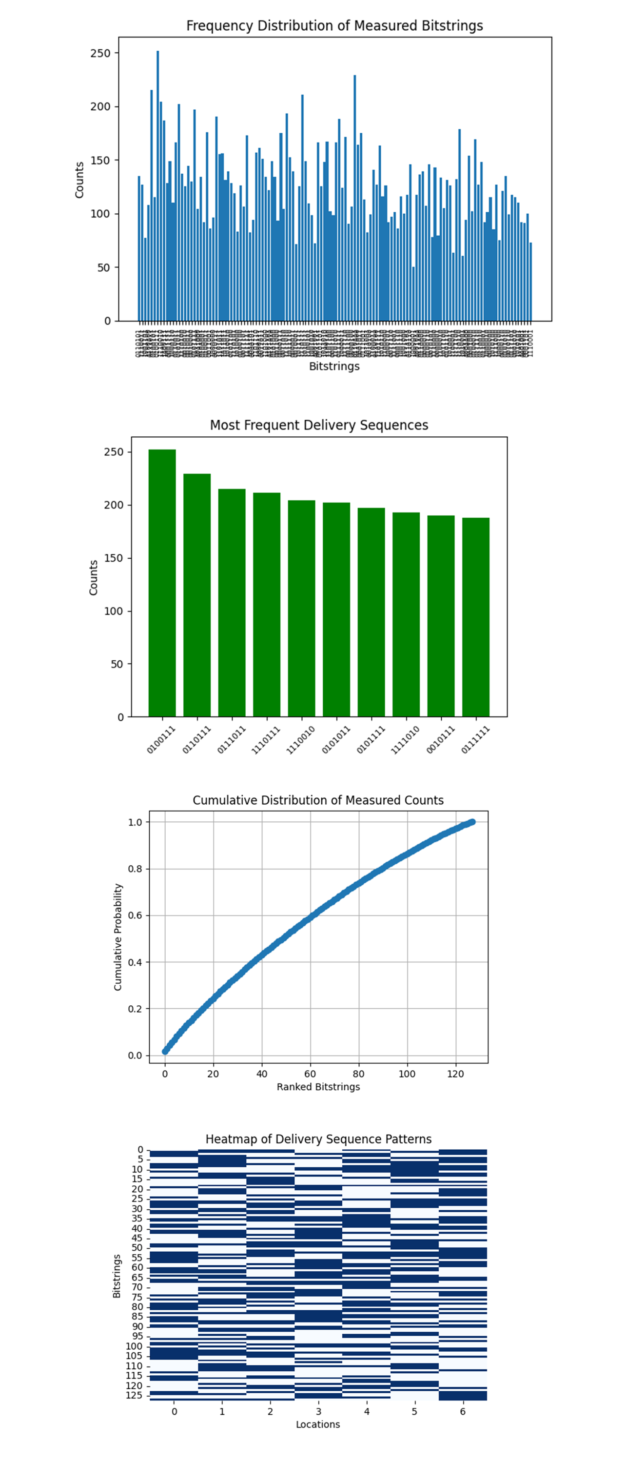
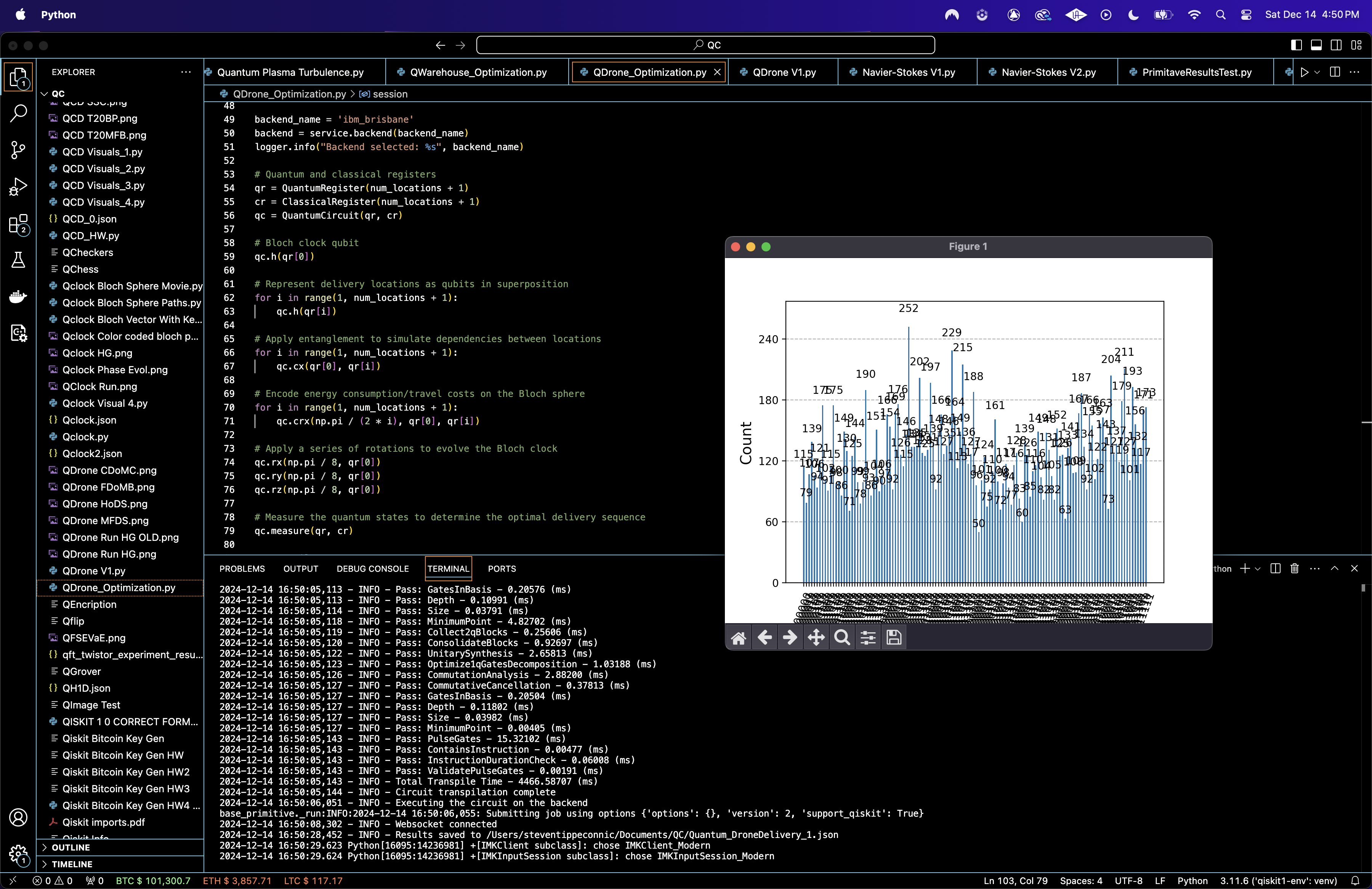
A histogram is plotted to visualize the frequency distribution of potential routes.

Results:
{
"raw_counts": {
"0110101": 135,
"1110011": 127,
"1001101": 77,
"1100100": 108,
"0111011": 215,
"0100101": 115,
"0100111": 252,
"1110010": 204, ... }
The bitstring 0100111 appears the most frequently, with a count of 252. This indicates that the algorithm consistently identifies this route as highly probable or optimal. Similarly, routes like 0111011 (215 counts) and 0110111 (229 counts) are also highly favored, pointing to a pattern of preferred routes among the measurements.
While certain routes dominate the measurements, there is a significant spread across other bitstrings, suggesting that the algorithm explores a diverse solution space. For example, routes like 1000001 and 1110001 have low counts (50 and 73), indicating that they are less optimal but still considered during the computation.

The Frequency Distribution of Measured Bitstrings above (code below) shows the counts of all measured bitstrings, representing potential drone delivery routes. There is a clear variance in frequency, with some routes appearing significantly more often than others. The distribution tapers off as we move toward less frequent routes, suggesting that the quantum algorithm focuses on a subset of routes it deems more optimal.
The Most Frequent Delivery Sequences above (code below) shows the top 10 most frequently measured bitstrings and their corresponding counts. Bitstring 0100111 dominates the measurements, with 252 counts, followed by 0111011 and 0110111 with 229 and 215 counts. These top 10 sequences represent the most likely optimal delivery routes, which drones can prioritize. By focusing on these routes, we can reduce computational overhead and streamline drone operations while maintaining high efficiency.
The Cumulative Distribution of Measured Counts above (code below) shows how the measured counts accumulate across all ranked bitstrings. The steep initial slope indicates that a small number of routes account for a large portion of the total measurements. The curve flattens as we include less frequent routes, which contribute minimally to the overall probability distribution. The quantum algorithm effectively concentrates on a small subset of highly probable routes, aligning with the goal of identifying optimal solutions efficiently.
The Heatmap of Delivery Sequence Patterns above (code below) visualizes the inclusion of locations (columns) across the most frequently measured bitstrings (rows).A 1 (dark blue) indicates that a location is included in the route, while a 0 (white) indicates it is skipped. Patterns in the heatmap reveal commonalities in which locations are visited together across different routes. Certain locations are consistently included in the top routes, suggesting that they are critical delivery points with high priority. Other locations appear sporadically, reflecting flexibility in optimizing drone energy consumption or accommodating variable delivery demands.

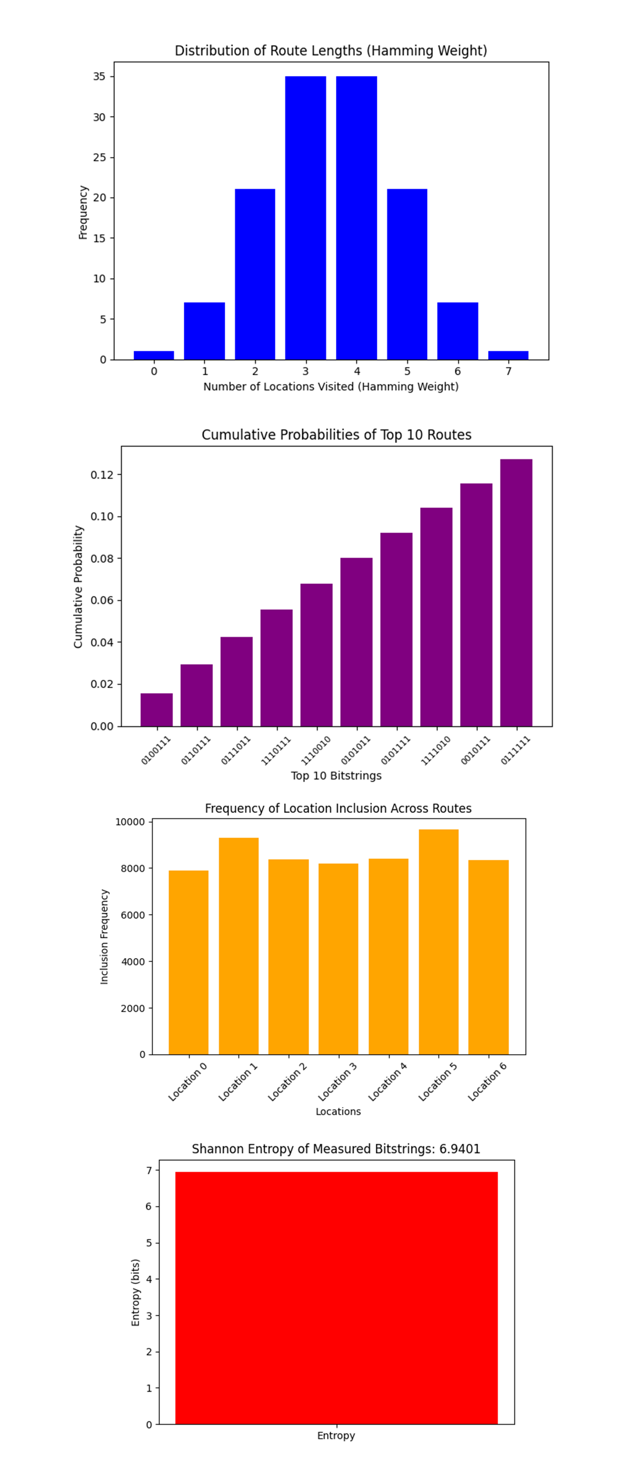
The Distribution of Route Lengths (Hamming Weight) above (code below) shows the distribution of routes based on the number of locations visited (Hamming weight of bitstrings). The peak at 3 - 4 locations indicates that the quantum optimization algorithm favored routes that visited a moderate number of locations rather than extremes (all locations or none). This suggests that the cost function encoded in the circuit balances efficiency with coverage. Drones are optimized to visit a reasonable number of locations without overextending, which could save energy and time.
The Cumulative Probabilities of Top 10 Routes above (code below) shows that the cumulative probabilities of the top 10 routes show a gradual increase, indicating that no single route dominates. Instead, multiple routes have comparable probabilities of being optimal. This highlights flexibility in route selection. Drones could choose from several near optimal paths based on real world constraints (weather, traffic, etc).
The Frequency of Location Inclusion Across Routes above (code below) shows how frequently each location was included in the measured routes. Locations 1, 4, and 5 appear more frequently, suggesting they are central to most optimal routes. Locations with higher inclusion frequencies may correspond to high priority delivery points (densely populated areas or critical delivery hubs). This data could inform drone fleet allocation to ensure these locations are consistently covered.
In the Shannon Entropy of Measured Bitstrings above (code below), the Shannon entropy value of ~6.94 bits indicates high diversity in the bitstring distribution, meaning the quantum algorithm explored a wide range of routes. High entropy reflects a large exploration of the solution space, ensuring that the algorithm did not prematurely converge on suboptimal solutions. This ensures fairness and flexibility in drone route planning.

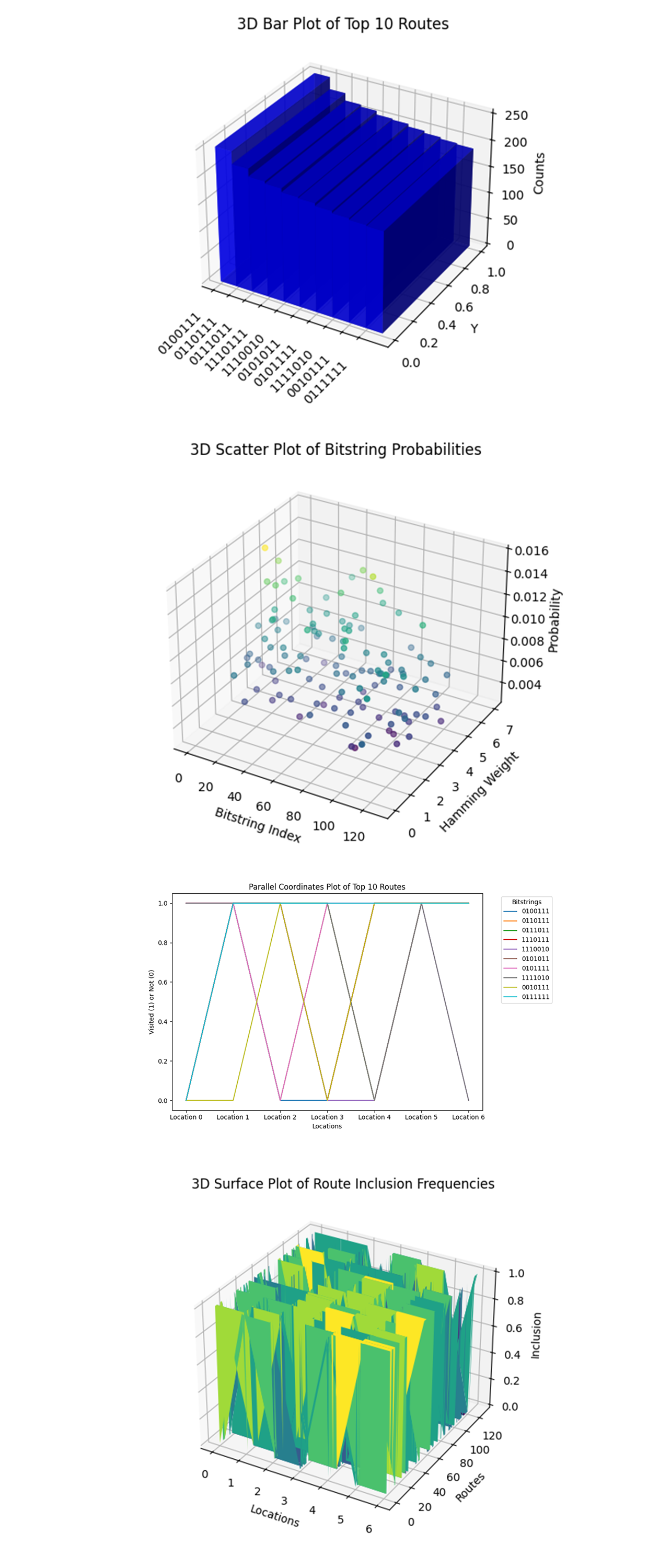
The 3D Bar Plot of Top 10 Routes above (code below) shows the top 10 bitstrings (routes) with their respective counts. The counts represent how often these routes appeared in the measurements, indicating their likelihood of being optimal.
The 3D Scatter Plot of Bitstring Probabilities above (code below) visualizes the probabilities of each bitstring (route) based on the measurements. It correlates the Hamming weight (number of locations visited) with the probability of the route. Routes with moderate Hamming weights (3 - 4 visited locations) have higher probabilities, indicating an optimized balance between energy consumption and coverage.
The Parallel Coordinates Plot of Top 10 Routes above (code below) shows the relationship between locations visited (1) or not (0) for the top 10 routes. Each line corresponds to a bitstring, and its path indicates whether a location is included in the route. This helps visualize which locations are commonly included or skipped in the top routes. High overlap in certain paths suggests key delivery hubs or regions that are critical in the optimization problem.
The 3D Surface Plot of Route Inclusion Frequencies above (code below) shows the inclusion frequencies of locations across all routes. Peaks in the plot indicate locations that are consistently included in many routes, while valleys represent less visited areas. High inclusion locations could correspond to high priority areas or regions with higher delivery demand.
In the end, the experiment successfully explored drone route optimization using quantum computing. By representing delivery locations as qubits and encoding travel distances and constraints, this circuit used quantum entanglement and superposition to evaluate multiple potential routes simultaneously. The optimization problem was designed to balance coverage (number of locations visited) with efficiency (energy consumption and travel time). The results gave the most efficient routes, the most frequently selected routes, key delivery hubs, and overall trends in the optimization process.

Code:


# Imports
# Imports
import numpy as np
import json
import pandas as pd
import logging
from qiskit import QuantumCircuit, QuantumRegister, ClassicalRegister, transpile
from qiskit_ibm_runtime import QiskitRuntimeService, Session, SamplerV2
from qiskit.visualization import plot_histogram
import matplotlib.pyplot as plt
from collections import Counter

# Logging
logging.basicConfig(level=logging. INFO, format='%(asctime)s - %(levelname)s - %(message)s')
logger = logging.getLogger(__name__)

# Load calibration data
def load_calibration_data(file_path):
    logger. info("Loading calibration data from %s", file_path)
    calibration_data = pd. read_csv(file_path)
    calibration_data.columns = calibration_data.columns.str.strip()  
    logger. info("Calibration data loaded successfully")
    return calibration_data

# Parse calibration data
def select_best_qubits(calibration_data, n_qubits):
    logger. info("Selecting the best qubits based on T1, T2, and error rates")
    print("Calibration data columns:", calibration_data.columns)
    qubits_sorted = calibration_data.sort_values(by=['√x (sx) error', 'T1 (us)', 'T2 (us)'], ascending=[True, False, False])
    best_qubits = qubits_sorted['Qubit'].head(n_qubits).tolist()
    logger. info("Selected qubits: %s", best_qubits)
    return best_qubits

# Load backend calibration data
calibration_file = '/Users/Downloads/ibm_brisbane_calibrations_2024-12-14T21_59_06Z.csv'
calibration_data = load_calibration_data(calibration_file)

# Select the best qubits based on T1, T2, and error rates
num_locations = 6  
best_qubits = select_best_qubits(calibration_data, num_locations + 1)

# IBMQ 
logger. info("Setting up IBM Q service")
service = QiskitRuntimeService(
    channel='ibm_quantum',
    instance='ibm-q/open/main',
    token='YOUR_IBMQ_API_KEY_O-`'
)

backend_name = 'ibm_brisbane'
backend = service.backend(backend_name)
logger. info("Backend selected: %s", backend_name)

# Quantum and classical registers
qr = QuantumRegister(num_locations + 1)  
cr = ClassicalRegister(num_locations + 1)
qc = QuantumCircuit(qr, cr)

# Bloch clock qubit
qc.h(qr[0])  

# Represent delivery locations as qubits in superposition
for i in range(1, num_locations + 1):
    qc.h(qr[i])  

# Apply entanglement to simulate dependencies between locations
for i in range(1, num_locations + 1):
    qc. cx(qr[0], qr[i])  

# Encode energy consumption/travel costs on the Bloch sphere
for i in range(1, num_locations + 1):
    qc.crx(np.pi / (2 * i), qr[0], qr[i])  

# Apply a series of rotations to evolve the Bloch clock
qc.rx(np.pi / 8, qr[0])  
qc.ry(np.pi / 8, qr[0])  
qc.rz(np.pi / 8, qr[0])  

# Measure the quantum states to determine the optimal delivery sequence
qc.measure(qr, cr)

# Transpile 
logger. info("Transpiling the quantum circuit for the backend")
qc_transpiled = transpile(qc, backend=backend, optimization_level=3)
logger. info("Circuit transpilation complete")

# Execute 
shots = 16384  
with Session(service=service, backend=backend) as session:
    sampler = SamplerV2(session=session)
    logger. info("Executing the circuit on the backend")
    job = sampler. run([qc_transpiled], shots=shots)
    job_result = job.result()

    # Results
    pub_results = job_result._pub_results[0]['__value__']
    data = pub_results['data']
    bit_array = data['c0']
    bitstrings = bit_array.get_bitstrings()  
    counts = dict(Counter(bitstrings))  

    # Save json
    results_data = {"raw_counts": counts}
    file_path = '/Users/Documents/Quantum_DroneDelivery_1.json'
    with open(file_path, 'w') as f:
        json.dump(results_data, f, indent=4)
    logger. info("Results saved to %s", file_path)

# Visualization
plot_histogram(counts)
plt. show()

//////////////////

Code for All Visuals
# Imports
import json
import matplotlib.pyplot as plt
from collections import Counter
import numpy as np
import seaborn as sns
from scipy.stats import entropy
from mpl_toolkits.mplot3d import Axes3D

# Load Run Results
file_path = '/Users/Documents/QC/Quantum_DroneDelivery_1.json'
with open(file_path, 'r') as file:
    data = json.load(file)

counts = data['raw_counts']
total_counts = sum(counts.values())

# Histogram of Bitstring Counts
def plot_histogram_counts(counts):
    plt. bar(counts.keys(), counts.values())
    plt.xlabel('Bitstrings')
    plt.ylabel('Counts')
    plt.title('Frequency Distribution of Measured Bitstrings')
    plt.xticks(rotation=90, fontsize=6)
    plt.tight_layout()
    plt.s how()

# Most Frequent Routes
def plot_top_routes(counts, top_n=10):
    sorted_counts = Counter(counts).most_common(top_n)
    bitstrings, freqs = zip(*sorted_counts)
    plt. bar(bitstrings, freqs, color='green')
    plt.xlabel('Top 10 Bitstrings')
    plt.ylabel('Counts')
    plt.title('Most Frequent Delivery Sequences')
    plt.xticks(rotation=45, fontsize=8)
    plt. show()

# Cumulative Distribution of Counts
def plot_cumulative_distribution(counts):
    total_counts = sum(counts.values())
    sorted_counts = sorted(counts.values(), reverse=True)
    cumulative = np.cumsum(sorted_counts) / total_counts
    plt.plot(range(len(cumulative)), cumulative, marker='o')
    plt.xlabel('Ranked Bitstrings')
    plt.ylabel('Cumulative Probability')
    plt.title('Cumulative Distribution of Measured Counts')
    plt.grid()
    plt. show()

# Heatmap of Bitstring Patterns
def plot_heatmap_patterns(counts):
    bitstrings = list(counts.keys())
    bit_array = np.array([list(map(int, bit)) for bit in bitstrings])
    sns.heatmap(bit_array, cmap='Blues', cbar=False)
    plt.xlabel('Locations')
    plt.ylabel('Bitstrings')
    plt.title('Heatmap of Delivery Sequence Patterns')
    plt. show()

# Call the visualization functions
plot_histogram_counts(counts)
plot_top_routes(counts)
plot_cumulative_distribution(counts)
plot_heatmap_patterns(counts)

# Distribution of Route Lengths (Hamming Weight)
def plot_route_length_distribution(counts):
    bitstrings = list(counts.keys())
    hamming_weights = [sum(map(int, bit)) for bit in bitstrings]  # Calculate Hamming weight for each bitstring
    weight_counts = Counter(hamming_weights)
    plt. bar(weight_counts.keys(), weight_counts.values(), color='blue')
    plt.xlabel('Number of Locations Visited (Hamming Weight)')
    plt.ylabel('Frequency')
    plt.title('Distribution of Route Lengths (Hamming Weight)')
    plt.xticks(range(max(weight_counts.keys()) + 1))
    plt.tight_layout()
    plt. show()

# Top 10 Routes with Cumulative Probabilities
def plot_top_10_cumulative_probabilities(counts):
    sorted_counts = Counter(counts).most_common(10)
    bitstrings, freqs = zip(*sorted_counts)
    cumulative_probs = np.cumsum([freq / total_counts for freq in freqs])
    plt. bar(range(len(bitstrings)), cumulative_probs, tick_label=bitstrings, color='purple')
    plt.xlabel('Top 10 Bitstrings')
    plt.ylabel('Cumulative Probability')
    plt.title('Cumulative Probabilities of Top 10 Routes')
    plt.xticks(rotation=45, fontsize=8)
    plt.tight_layout()
    plt. show()

# Distribution of Route Inclusion Frequencies
def plot_location_inclusion_frequency(counts):
    bitstrings = list(counts.keys())
    inclusion_matrix = np.array([list(map(int, bit)) for bit in bitstrings])
    location_inclusion = inclusion_matrix.T @ np.array(list(counts.values()))
    plt. bar(range(len(location_inclusion)), location_inclusion, color='orange')
    plt.xlabel('Locations')
    plt.ylabel('Inclusion Frequency')
    plt.title('Frequency of Location Inclusion Across Routes')
    plt.xticks(range(len(location_inclusion)), [f"Location {i}" for i in range(len(location_inclusion))], rotation=45)
    plt.tight_layout()
    plt. show()

# Entropy of the Bitstring Distribution
def plot_entropy_of_distribution(counts):
    normalized_probs = np.array([count / total_counts for count in counts.values()])
    entropy_value = entropy(normalized_probs, base=2)
    plt. bar(["Entropy"], [entropy_value], color='red')
    plt.title(f'Shannon Entropy of Measured Bitstrings: {entropy_value:.4f}')
    plt.ylabel('Entropy (bits)')
    plt. show()

# Call the visualization functions
plot_route_length_distribution(counts)
plot_top_10_cumulative_probabilities(counts)
plot_location_inclusion_frequency(counts)
plot_entropy_of_distribution(counts)

# 3D Bar Plot of Top 10 Routes
def plot_3d_bar_top_routes(counts):
    sorted_counts = Counter(counts).most_common(10)
    bitstrings, freqs = zip(*sorted_counts)

    fig = plt.figure()
    ax = fig.add_subplot(111, projection='3d')

    xpos = np.arange(len(bitstrings))
    ypos = np.zeros(len(bitstrings))
    zpos = np.zeros(len(bitstrings))

    dx = np.ones(len(bitstrings))
    dy = np.ones(len(bitstrings))
    dz = freqs

    ax.bar3d(xpos, ypos, zpos, dx, dy, dz, color='blue', alpha=0.7)

    ax.set_xticks(xpos)
    ax.set_xticklabels(bitstrings, rotation=45, ha='right')
    ax.set_xlabel('')
    ax.set_ylabel('Y')
    ax.set_zlabel('Counts')
    ax.set_title('3D Bar Plot of Top 10 Routes')

    plt.tight_layout()
    plt. show()

# 3D Scatter Plot of Bitstring Probabilities
def plot_3d_scatter_probabilities(counts):
    bitstrings = list(counts.keys())
    probabilities = [count / total_counts for count in counts.values()]
    hamming_weights = [sum(map(int, bit)) for bit in bitstrings]

    fig = plt.figure()
    ax = fig.add_subplot(111, projection='3d')

    x = np.arange(len(bitstrings))
    y = hamming_weights
    z = probabilities

    ax.scatter(x, y, z, c=z, cmap='viridis', depthshade=True)

    ax.set_xlabel('Bitstring Index')
    ax.set_ylabel('Hamming Weight')
    ax.set_zlabel('Probability')
    ax.set_title('3D Scatter Plot of Bitstring Probabilities')

    plt.tight_layout()
    plt. show()

# Parallel Coordinates Plot of Top 10 Routes
def plot_parallel_coordinates_top_routes(counts):
    sorted_counts = Counter(counts).most_common(10)
    bitstrings, freqs = zip(*sorted_counts)

    data = np.array([list(map(int, bit)) for bit in bitstrings])
    fig, ax = plt.subplots()
    for row, label in zip(data, bitstrings):
        ax.plot(range(len(row)), row, label=label)

    ax.set_xticks(range(data.shape[1]))
    ax.set_xticklabels([f"Location {i}" for i in range(data.shape[1])])
    ax.set_xlabel("Locations")
    ax.set_ylabel("Visited (1) or Not (0)")
    ax.set_title("Parallel Coordinates Plot of Top 10 Routes")
    plt.legend(loc='upper left', bbox_to_anchor=(1.05, 1), title="Bitstrings")
    plt.tight_layout()
    plt. show()

# 3D Surface Plot of Route Inclusion Frequencies
def plot_3d_surface_inclusion(counts):
    bitstrings = list(counts.keys())
    inclusion_matrix = np.array([list(map(int, bit)) for bit in bitstrings])
    inclusion_frequency = inclusion_matrix.T @ np.array(list(counts.values()))

    x = np.arange(inclusion_matrix.shape[1])  # Locations
    y = np.arange(inclusion_matrix.shape[0])  # Routes
    X, Y = np.meshgrid(x, y)
    Z = inclusion_matrix

    fig = plt.figure()
    ax = fig.add_subplot(111, projection='3d')
    ax.plot_surface(X, Y, Z, cmap='viridis', edgecolor='none')

    ax.set_xlabel('Locations')
    ax.set_ylabel('Routes')
    ax.set_zlabel('Inclusion')
    ax.set_title('3D Surface Plot of Route Inclusion Frequencies')

    plt. show()

# Call the visualization functions
plot_3d_bar_top_routes(counts)
plot_3d_scatter_probabilities(counts)
plot_parallel_coordinates_top_routes(counts)
plot_3d_surface_inclusion(counts)

# End