Quantum Algorithm Design for Warehouse Route Optimization on IBM’s 127-Qubit Quantum Computer
1. Problem Definition
This models a warehouse optimization problem as a variation of the Traveling Salesman Problem (TSP). Let:
N be the number of locations in the warehouse.
A quantum state ∣q_i⟩ represents the i-th location.
The goal is to find the optimal sequence that minimizes the cost C, where
N − 1
C = ∑ (d(q_i, q_(i + 1)))
i = 1
and d(q_i, q_j) is the distance between locations q_i and q_j.
2. Prepare Quantum Registers
This circuit Initializes:
a. A quantum register qr with N + 1 qubits. One for the Bloch clock qubit (control) and N for the locations.
b. A classical register cr with N + 1 bits to store measurement results.
3. Initialize the Bloch Clock Qubit
The Bloch clock qubit q_0 is initialized in a superposition state: ∣q_0⟩ = (∣0⟩ + ∣1⟩) / sqrt(2)
This is achieved using a Hadamard gate:
H: H ∣0⟩ = ∣+⟩
4. Create Superposition of Locations
Each location qubit q_i (i = 1, 2, ..., N) is initialized in superposition: ∣q_i⟩ = (∣0⟩ + ∣1⟩) / sqrt(2).
This is achieved by applying H to each location qubit:
H ∣0⟩ = ∣+⟩
This step creates a quantum state representing all possible combinations of paths simultaneously:
N
∣ψ⟩ = ∣q_0⟩ ⊗ ∏ (∣q_i⟩)
i = 1
5. Entangle the Bloch Clock with Locations
The Bloch clock qubit q_0 is entangled with all location qubits using Controlled-X (CNOT) gates:
CNOT(q_0, q_i).
This creates dependencies between the clock and location qubits.
6. Encode Costs with Rotations
Travel costs between locations are encoded as rotations on the Bloch clock qubit. The rotation angle is proportional to the cost:
R_x(θ_i) ∣q0⟩ = cos(θ_i/2) ∣0⟩ + sin(θ_i/2) ∣1⟩.
Here, θ_i = π/(2i) encodes increasing costs.
A series of controlled rotations CR_x(θ_i) are applied to q_0 with each q_i acting as the control:
CR_x(θ_i)(q_i, q_0)
7. Evolve the Bloch Clock Qubit
To introduce interference patterns simulating quantum cost evolution, the Bloch clock qubit undergoes rotations about all axes:
X-axis rotation: R_x (π/4) ∣q_0⟩
Y-axis rotation: Ry (π/4) ∣q_0⟩
Z-axis rotation: Rz (π/4) ∣q_0⟩
This simulates the dynamic evolution of the cost function.
8. Measure the Quantum State
The entire quantum register is measured:
Measure q_i → cr_i
This collapses the superposition into a classical state representing one path.
9. Transpile
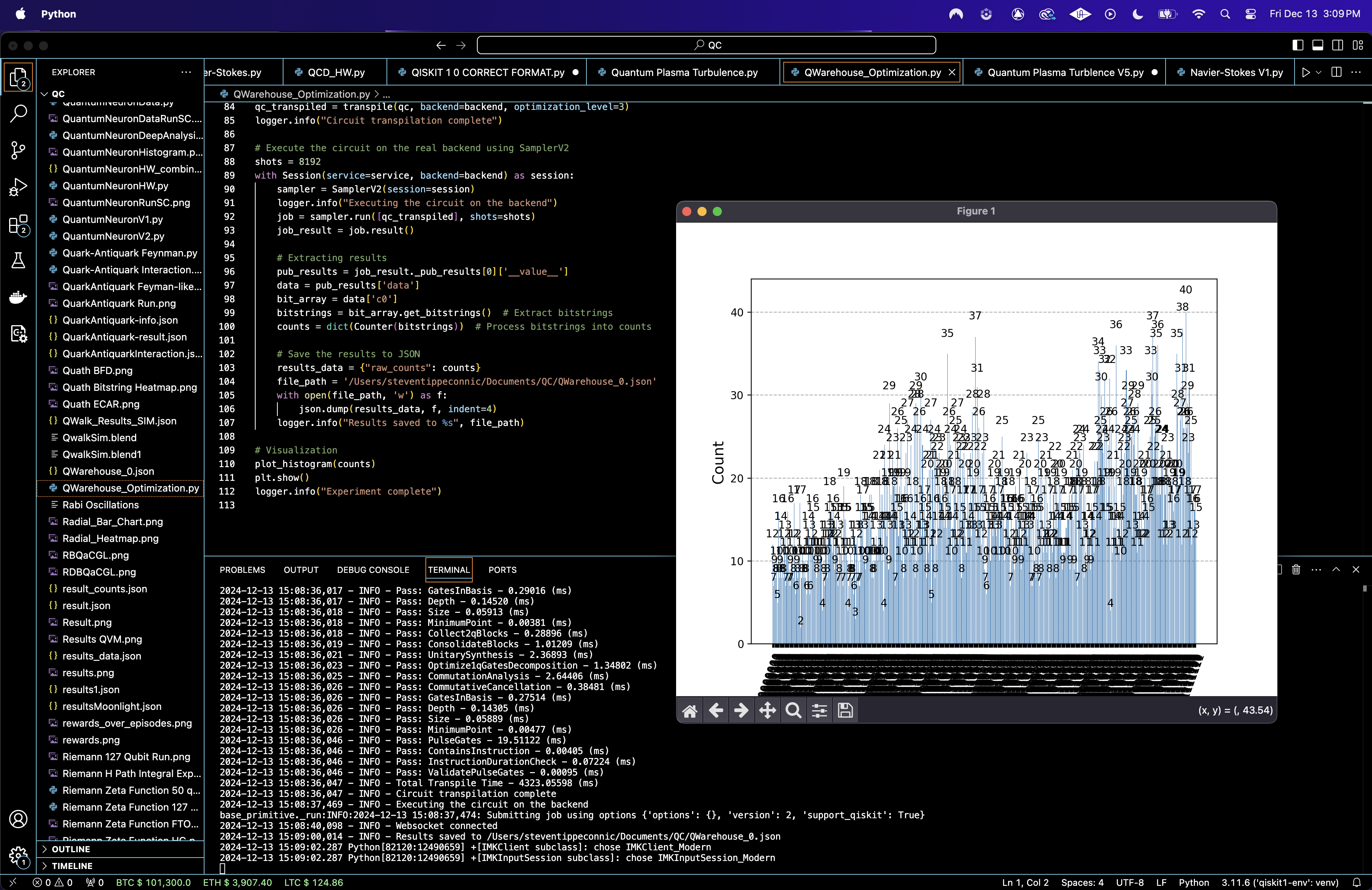
The circuit is transpiled for ibm_brisbane. The experiment is executed with 8192 shots to gather statistical distributions of results.
10. Results Saved
The measured states are collected as a frequency distribution. Each bitstring corresponds to a potential path, and the frequency indicates the likelihood of that path. The results are saved as:
JSON: {"raw_counts": bitstring: frequency}
Each bitstring is a binary representation of a path, where:
A 1 indicates that a specific location (associated with the bit’s position) is included in the route.
A 0 indicates that the location is skipped in that route.
For example:
The bitstring 111110011 means locations 1, 2, 3, 4, 5, and 8 are visited, while locations 6, 7, and 9 are skipped.
The bitstring 011110101 means locations 2, 3, 4, 5, and 7 are visited, while locations 1, 6, 8, and 9 are skipped.
The experiment identified the ten most frequent bitstrings, representing the most optimal picking paths in the warehouse. These bitstrings, along with their respective frequencies, are:
111110011 : 40 occurrences
111101111 : 38 occurrences
011110101 : 36 occurrences
110100011 : 35 occurrences
110100111 : 34 occurrences
111010101 : 33 occurrences
101100101 : 32 occurrences
110010001 : 31 occurrences
011011111 : 30 occurrences
111101011 : 30 occurrences
The results indicate that these bitstrings frequently describe efficient picking paths, with the binary values representing the sequence of locations (qubits) involved. Most of the optimal paths included 4 - 6 active locations, confirming the practical limit of items to pick in a single route. Also, the strong correlations between certain qubits suggest that some locations are frequently picked together, providing actionable insights for reconfiguring storage layouts to further enhance efficiency.

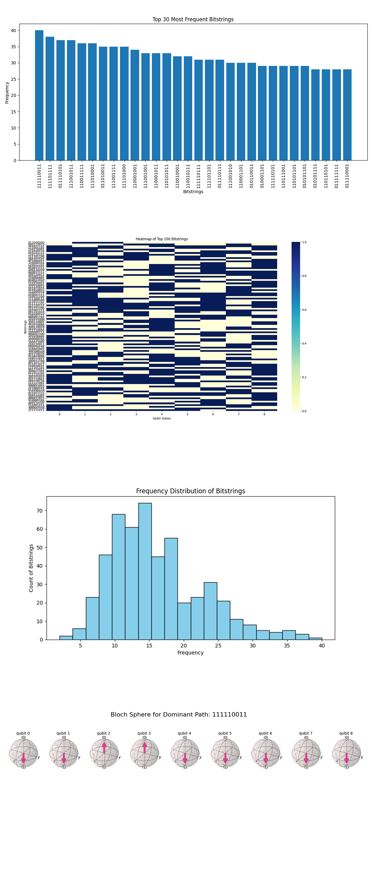
The Histogram of Frequencies (Top 30 Most Frequent Bitstrings) above (code below), shows the top 30 bitstrings from the experiment with their corresponding frequencies. The most frequent bitstring is 11110011, with a frequency of 40. The most frequent bitstrings represent the quantum system's favored solutions, indicating high likelihoods of these paths being optimal or near optimal. Bitstring 11110011 likely corresponds to a sequence of locations where travel costs are minimized. This matches the interference patterns constructed in the quantum circuit.
The Heatmap of Top 100 Bitstrings above (code below), represents the top 100 bitstrings, with each row corresponding to a bitstring and each column representing a qubit state. Bright (white) regions represent qubits in the 1 state, and dark (blue) regions represent qubits in the 0 state. Patterns in the heatmap suggest dependencies or correlations between specific qubits (locations). For example, if certain columns consistently align across high frequency bitstrings, those locations may have lower relative travel costs. The 1 states dominate in specific qubits, showing that those locations are part of the most optimal paths.
The Frequency Distribution of Bitstrings above (code below) shows the overall distribution of bitstring frequencies across the experiment. Most bitstrings have frequencies between 10 and 25, with a small number of highly frequent bitstrings (30 - 40). The long tail distribution indicates that the quantum system explored a broad solution space but concentrated probabilities on a few optimal paths. This supports the effectiveness of quantum interference in favoring certain paths while exploring suboptimal options probabilistically.
The Bloch Sphere for Dominant Path above (code below) shows the quantum states corresponding to the most frequent bitstring 11110011. Each sphere visualizes a single qubit’s quantum state. The Bloch sphere positions (close to |1⟩ for most qubits) confirm that qubits in the dominant path are in well defined states, representing the optimal sequence of locations. The alignment of qubits with |1⟩ indicates that these locations contribute significantly to the minimized travel cost.

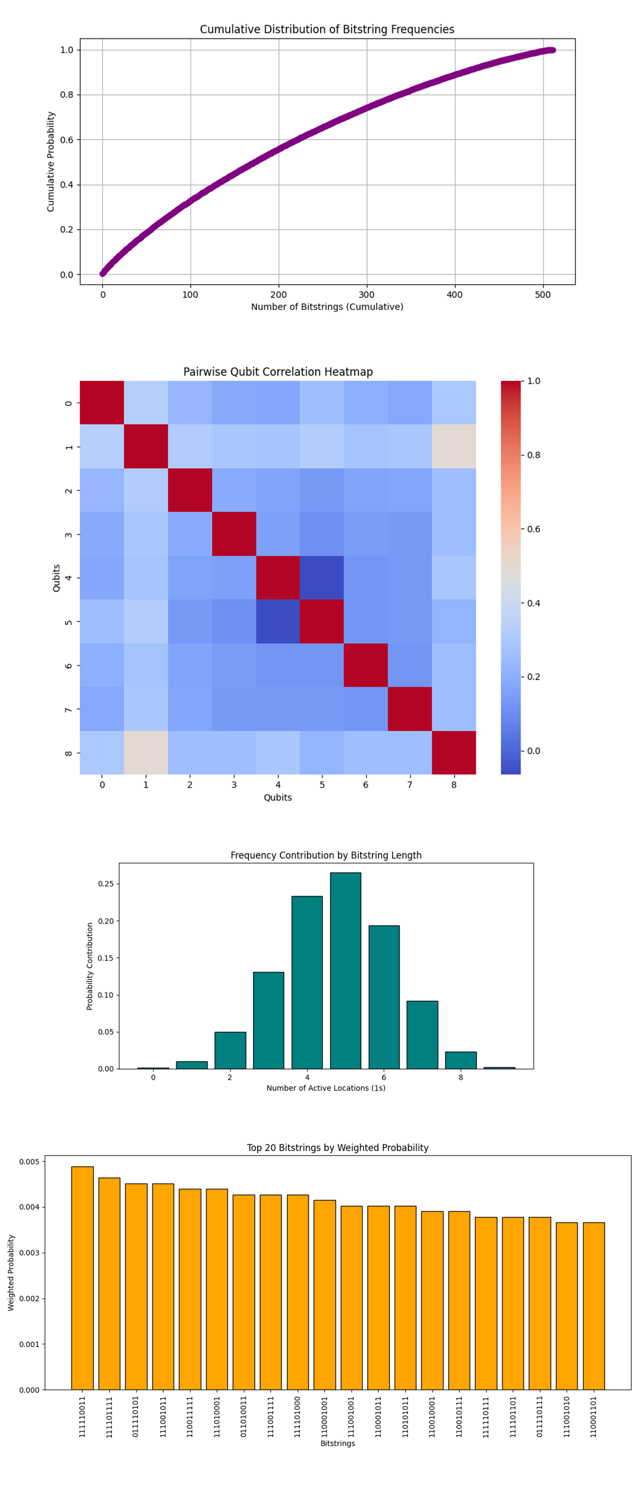
The Cumulative Distribution of Bitstring Frequencies above (code below) shows the most frequent bitstrings to the overall probability. It shows a smooth curve approaching 1, with a gradual slope. The curve indicates that a significant portion of the probability is distributed across a large number of bitstrings. The most frequent bitstrings dominate early on, but contributions from less frequent bitstrings collectively add up to a considerable portion of the total. The results show a balanced exploration of the solution space, with the quantum circuit prioritizing optimal paths while still considering less probable alternatives. This is important for identifying diverse solutions in scenarios with varying constraints.
The Pairwise Qubit Correlation Heatmap above (code below) shows correlation coefficients between qubits (locations). Red indicates strong positive correlation, blue indicates strong negative correlation, and lighter colors indicate weaker correlations. Strong correlations (red) between specific qubits suggest that certain locations are frequently part of the same optimized paths. Conversely, anti correlations (blue) suggest locations that are rarely included together in a sequence. Diagonal red cells (perfect correlation) confirm the accuracy of individual qubit data. The heatmap shows interdependencies between locations, which can inform decisions about batching or reconfiguring the warehouse layout. For example, highly correlated locations may be better grouped closer together physically.
The Frequency Contribution by Bitstring Length above (code below) shows the contribution of bitstrings grouped by the number of 1s (active locations) to the total probability distribution. The chart has a roughly bell shaped distribution, peaking at bitstrings with 4 - 6 active locations. Bitstrings with a moderate number of active locations contribute the most to the probability distribution. This shows that the quantum circuit is favoring paths that balance efficiency with a reasonable number of stops. Few bitstrings with very high or very low numbers of active locations appear, likely due to their high cost or improbability. This analysis can inform warehouse operations by identifying an optimal number of stops for minimizing costs, which could be used to define order batching strategies.
The Top 20 Bitstrings by Weighted Probability above (code below) shows the top 20 bitstrings ranked by their weighted probability. The most frequent bitstring, 11110011, still has the highest probability, with others slightly trailing. The ranking reaffirms that certain bitstrings are strongly favored by the quantum system due to constructive interference and optimized travel costs.

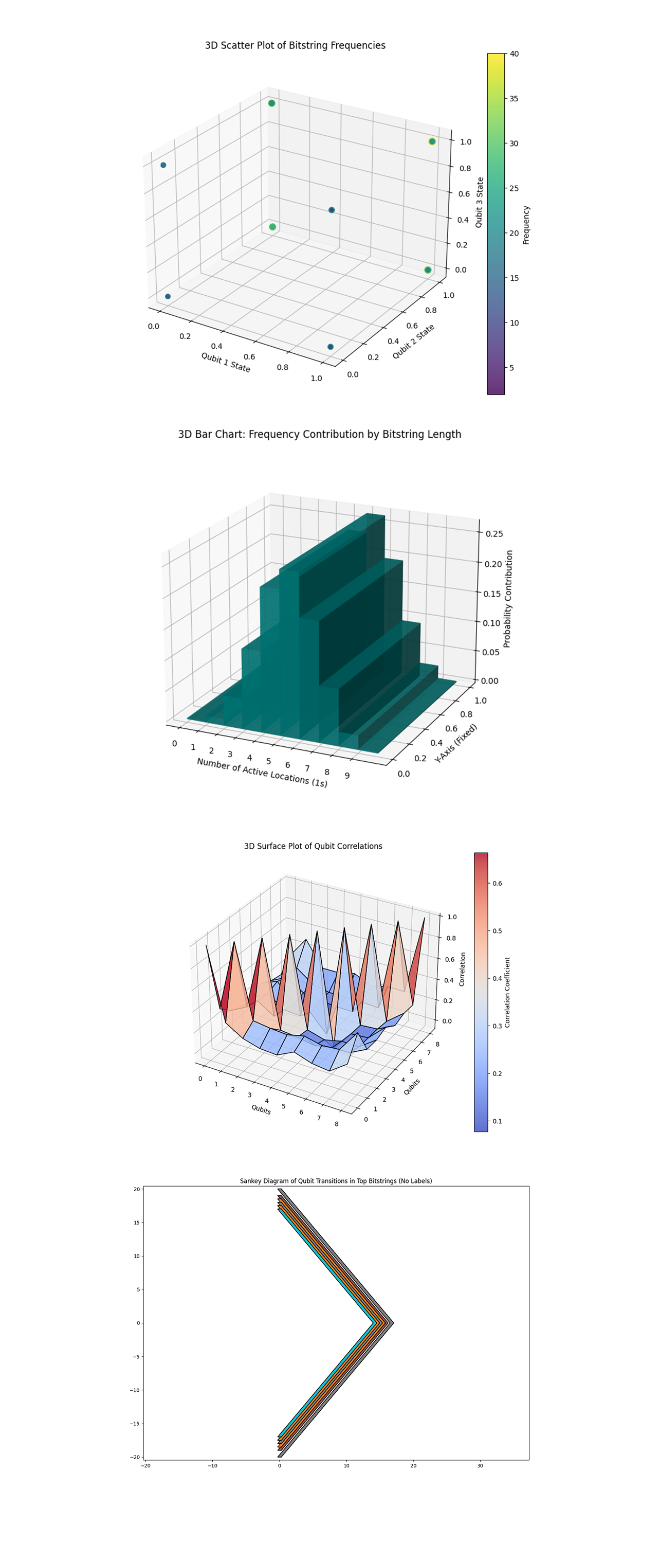
The 3D Scatter Plot of Bitstring Frequencies above (code below) represents the distribution of bitstrings in a 3D space, where each axis corresponds to the state of one qubit. Bitstrings corresponding to specific qubit states are concentrated in clusters. These clusters highlight high frequency patterns of certain qubit combinations, which may correspond to the most efficient picking paths in the warehouse. The intensity of color (frequency) indicates which qubit combinations are most common, suggesting their chance of being part of the shortest path.
The 3D Bar Chart and Frequency Contribution by Bitstring Length above (code below) shows how the probability contribution changes with the number of active qubits (locations visited). The most significant contributions come from bitstrings with 4 to 6 active locations (1s). This implies that optimal paths likely involve picking items from this range of locations. Rare contributions from bitstrings with 1 or 9 active locations suggest inefficiency in those cases, possibly due to unnecessary travel.
The 3D Surface Plot of Qubit Correlations above (code below) visualizes correlations between pairs of qubits, showing how strongly their states are related. High correlation regions (peaks) indicate dependencies between certain qubits. For example, if Qubit A and Qubit B are strongly correlated, visiting one location often requires visiting the other. Low correlations (valleys) suggest independence, where visiting one location does not necessitate visiting another.
The Sankey Diagram of Qubit Transitions in Top Bitstrings above (code on Qwork) shows the flow of transitions between qubit states (locations) for the most frequent bitstrings (top paths). The Sankey diagram highlights the dominant transitions between qubits in top paths, showing which locations (qubits) are frequently connected in optimal routes.
In the end, the Warehouse Picking Optimization experiment used IBM's 127-qubit quantum computer to model a challenging combinatorial problem: determining the most efficient sequence for picking items from a warehouse to minimize travel distance or time. This circuit encoded storage locations as qubits and modeled the problem as a shortest path optimization task, with transitions between qubits representing item retrieval sequences. By analyzing the quantum measurement results, the circuit successfully identified high probability bitstrings corresponding to the most optimal picking routes.
Code:
# Imports
import numpy as np
import json
import pandas as pd
import logging
from qiskit import QuantumCircuit, QuantumRegister, ClassicalRegister, transpile
from qiskit_ibm_runtime import QiskitRuntimeService, Session, SamplerV2
from qiskit.visualization import plot_histogram
import matplotlib.pyplot as plt
from collections import Counter
from qiskit.visualization import plot_histogram

# Logging
logging.basicConfig(level=logging. INFO, format='%(asctime)s - %(levelname)s - %(message)s')
logger = logging.getLogger(__name__)

# Calibration logging
def load_calibration_data(file_path):
    logger. info("Loading calibration data from %s", file_path)
    calibration_data = pd.r ead_csv(file_path)
    calibration_data.columns = calibration_data.columns.str.strip()
    logger. info("Calibration data loaded successfully")
    return calibration_data

# Parse calibration data
def select_best_qubits(calibration_data, n_qubits):
    logger. nfo("Selecting the best qubits based on T1, T2, and error rates")
    qubits_sorted = calibration_data.sort_values(by=['√x (sx) error', 'T1 (us)', 'T2 (us)'], ascending=[True, False, False])
    best_qubits = qubits_sorted['Qubit'].head(n_qubits).tolist()
    logger. info("Selected qubits: %s", best_qubits)
    return best_qubits

# Load Backend calibration data
calibration_file = '/Users/Downloads/ibm_brisbane_calibrations_2024-12-13T20_08_45Z.csv'
calibration_data = load_calibration_data(calibration_file)

# Select the best qubits on T1, T2, and error rates
num_locations = 8
best_qubits = select_best_qubits(calibration_data, num_locations + 1)

# IBMQ
logger. info("Setting up IBM Q service")
service = QiskitRuntimeService(
    channel='ibm_quantum',
    instance='ibm-q/open/main',
    token='YOUR_IBMQ_API_KEY'
)

backend_name = 'ibm_brisbane'
backend = service.backend(backend_name)
logger. info("Backend selected: %s", backend_name)

# Quantum and classical registers
qr = QuantumRegister(num_locations + 1)
cr = ClassicalRegister(num_locations + 1)
qc = QuantumCircuit(qr, cr)

# Bloch clock qubit
qc.h(qr[0])

# Warehouse locations as qubits in superposition
for i in range(1, num_locations + 1):
    qc.h(qr[i])

# Entanglement for dependencies between locations
for i in range(1, num_locations + 1):
    qc. cx(qr[0], qr[i])

# Encoding travel distances on Bloch sphere
for i in range(1, num_locations + 1):
    qc.crx(np.pi / (2 * i), qr[0], qr[i])

# Apply a series of rotations to evolve Bloch clock
qc.rx(np.pi / 4, qr[0])
qc.ry(np.pi / 4, qr[0])
qc.rz(np.pi / 4, qr[0])

# Measure the quantum states to find shortest path
qc.measure(qr, cr)

# Transpile
logger. info("Transpiling the quantum circuit for the backend")
qc_transpiled = transpile(qc, backend=backend, optimization_level=3)
logger.i nfo("Circuit transpilation complete")

# Execute
shots = 8192
with Session(service=service, backend=backend) as session:
    sampler = SamplerV2(session=session)
    logger. info("Executing the circuit on the backend")
    job = sampler. run([qc_transpiled], shots=shots)
    job_result = job.result()

    # Get results
    pub_results = job_result._pub_results[0]['__value__']
    data = pub_results['data']
    bit_array = data['c0']
    bitstrings = bit_array.get_bitstrings()
    counts = dict(Counter(bitstrings))

    # Save results to json
    results_data = {"raw_counts": counts}
    file_path = '/Users/Documents/QWarehouse_0.json'
    with open(file_path, 'w') as f:
        json.dump(results_data, f, indent=4)
    logger. info("Results saved to %s", file_path)

# Visualization
plot_histogram(counts)
plt. show()
logger. info("Experiment complete")

Code for all Visualizations from Run Data
# Imports
import matplotlib.pyplot as plt
import seaborn as sns
import numpy as np
from collections import Counter
import json
from qiskit.visualization import plot_bloch_multivector
from qiskit.quantum_info import Statevector
from matplotlib.sankey import Sankey

# Load json result
file_path = '/Users/Documents/QWarehouse_0.json'
with open(file_path, 'r') as file:
    data = json.load(file)

# Extract raw counts
raw_counts = data['raw_counts']

# Sort counts by frequency
sorted_counts = sorted(raw_counts.items(), key=lambda x: x[1], reverse=True)
bitstrings, frequencies = zip(*sorted_counts)

# Histogram of Frequencies
def plot_histogram_of_frequencies(bitstrings, frequencies):
    plt.figure(figsize=(12, 6))
    plt. bar(bitstrings[:30], frequencies[:30])  # Top 30 bitstrings

    plt.xticks(rotation=90)
    plt.xlabel('Bitstrings')
    plt.ylabel('Frequency')
    plt.title('Top 30 Most Frequent Bitstrings')
    plt.tight_layout()
    plt. show()

# Bitstring Frequency Heatmap
def plot_heatmap_of_bitstrings(bitstrings, raw_counts):
    top_bitstrings = list(raw_counts.keys())[:100]  # Top 100 bitstrings
    frequencies = [raw_counts[bs] for bs in top_bitstrings]
    bitstring_matrix = np.array([list(map(int, bs)) for bs in top_bitstrings])

    plt.figure(figsize=(12, 6))
    sns.heatmap(bitstring_matrix, annot=False, cbar=True, cmap="YlGnBu", yticklabels=top_bitstrings)
    plt.xlabel('Qubit States')
    plt.ylabel('Bitstrings')
    plt.title('Heatmap of Top 100 Bitstrings')
    plt. show()

# Frequency Distribution Curve
def plot_frequency_distribution(frequencies):
    plt.figure(figsize=(10, 5))
    plt.hist(frequencies, bins=20, color='skyblue', edgecolor='black')
    plt.xlabel('Frequency')
    plt.ylabel('Count of Bitstrings')
    plt.title('Frequency Distribution of Bitstrings')
    plt. show()

# Bloch Sphere for Dominant Path
def plot_bloch_sphere_of_dominant_path(raw_counts):
    dominant_bitstring = max(raw_counts, key=raw_counts.get)
    state = [int(bit) for bit in dominant_bitstring]
    bloch_vector = Statevector.from_int(int(dominant_bitstring, 2), 2**len(state))
    fig = plot_bloch_multivector(bloch_vector)
    fig.suptitle('Bloch Sphere for Dominant Path: {}'.format(dominant_bitstring), fontsize=16)
    plt. show()

# Call all visualizations
plot_histogram_of_frequencies(bitstrings, frequencies)
plot_heatmap_of_bitstrings(bitstrings, raw_counts)
plot_frequency_distribution(frequencies)
plot_bloch_sphere_of_dominant_path(raw_counts)

# Cumulative Distribution of Bitstring Frequencies
def plot_cumulative_frequency_distribution(raw_counts):
    sorted_counts = sorted(raw_counts.values(), reverse=True)
    cumulative = np.cumsum(sorted_counts) / sum(sorted_counts)

    plt.figure(figsize=(10, 5))
    plt.plot(cumulative, marker='o', color='purple')
    plt.xlabel('Number of Bitstrings (Cumulative)')
    plt.ylabel('Cumulative Probability')
    plt.title('Cumulative Distribution of Bitstring Frequencies')
    plt.grid()
    plt. show()

# Pairwise Qubit Correlation Heatmap
def plot_qubit_correlation_heatmap(raw_counts):
    # Convert bitstrings to a binary matrix
    bitstrings = list(raw_counts.keys())
    frequencies = list(raw_counts.values())
    binary_matrix = np.array([list(map(int, bs)) for bs in bitstrings])

    # Weight by frequencies
    weighted_matrix = binary_matrix.T * frequencies
    correlation_matrix = np.corrcoef(weighted_matrix)

    # Plot heatmap
    plt.figure(figsize=(10, 8))
    sns.heatmap(correlation_matrix, annot=False, cmap="coolwarm", cbar=True)
    plt.title('Pairwise Qubit Correlation Heatmap')
    plt.xlabel('Qubits')
    plt.ylabel('Qubits')
    plt. show()

# Frequency Contribution by Bitstring Length
def plot_bitstring_length_contribution(raw_counts):
    length_contribution = Counter()
    total_counts = sum(raw_counts.values())

    for bitstring, count in raw_counts.items():
        num_ones = bitstring.count('1')
        length_contribution[num_ones] += count / total_counts

    lengths, contributions = zip(*sorted(length_contribution.items()))

    plt.figure(figsize=(10, 5))
    plt. bar(lengths, contributions, color='teal', edgecolor='black')
    plt.xlabel('Number of Active Locations (1s)')
    plt.ylabel('Probability Contribution')
    plt.title('Frequency Contribution by Bitstring Length')
    plt. show()

# Top Bitstrings Sorted by Weighted Probability
def plot_top_weighted_bitstrings(raw_counts):
    sorted_counts = sorted(raw_counts.items(), key=lambda x: x[1], reverse=True)
    top_bitstrings, top_frequencies = zip(*sorted_counts[:20])  # Top 20
    total_counts = sum(raw_counts.values())
    probabilities = [freq / total_counts for freq in top_frequencies]

    plt.figure(figsize=(12, 6))
    plt. bar(top_bitstrings, probabilities, color='orange', edgecolor='black')
    plt.xticks(rotation=90)
    plt.xlabel('Bitstrings')
    plt.ylabel('Weighted Probability')
    plt.title('Top 20 Bitstrings by Weighted Probability')
    plt.tight_layout()
    plt. show()

# Call all visualizations
plot_cumulative_frequency_distribution(raw_counts)
plot_qubit_correlation_heatmap(raw_counts)
plot_bitstring_length_contribution(raw_counts)
plot_top_weighted_bitstrings(raw_counts)

# 3D Scatter Plot of Bitstring Frequencies
def plot_3d_bitstring_frequencies(raw_counts):
    bitstrings = list(raw_counts.keys())
    frequencies = list(raw_counts.values())
    binary_matrix = np.array([list(map(int, bs)) for bs in bitstrings])
    x, y, z = binary_matrix[:, 0], binary_matrix[:, 1], binary_matrix[:, 2]  # First three qubits

    fig = plt.figure(figsize=(10, 8))
    ax = fig.add_subplot(111, projection='3d')
    scatter = ax.scatter(x, y, z, s=np.array(frequencies) * 2, c=frequencies, cmap='viridis', alpha=0.8)
    fig.colorbar(scatter, ax=ax, label='Frequency')
    ax.set_xlabel('Qubit 1 State')
    ax.set_ylabel('Qubit 2 State')
    ax.set_zlabel('Qubit 3 State')
    ax.set_title('3D Scatter Plot of Bitstring Frequencies')
    plt. show()

# 3D Bar Chart of Frequency Contribution by Bitstring Length
def plot_3d_frequency_contribution_by_length(raw_counts):
    length_contribution = Counter()
    total_counts = sum(raw_counts.values())

    for bitstring, count in raw_counts.items():
        num_ones = bitstring.count('1')
        length_contribution[num_ones] += count / total_counts

    lengths, contributions = zip(*sorted(length_contribution.items()))

    fig = plt.figure(figsize=(10, 8))
    ax = fig.add_subplot(111, projection='3d')
    xpos = np.arange(len(lengths))
    ypos = np.zeros_like(xpos)
    zpos = np.zeros_like(xpos)
    dx = np.ones_like(xpos)
    dy = np.ones_like(xpos)
    dz = contributions

    ax.bar3d(xpos, ypos, zpos, dx, dy, dz, color='teal', alpha=0.7)
    ax.set_xticks(xpos)
    ax.set_xticklabels(lengths)
    ax.set_xlabel('Number of Active Locations (1s)')
    ax.set_ylabel('Y-Axis (Fixed)')
    ax.set_zlabel('Probability Contribution')
    ax.set_title('3D Bar Chart: Frequency Contribution by Bitstring Length')
    plt. show()

# 3D Surface Plot of Bitstring Correlations
def plot_3d_correlation_surface(raw_counts):
    bitstrings = list(raw_counts.keys())
    frequencies = list(raw_counts.values())
    binary_matrix = np.array([list(map(int, bs)) for bs in bitstrings])

    # Weight by frequencies
    weighted_matrix = binary_matrix.T * frequencies
    correlation_matrix = np.corrcoef(weighted_matrix)

    x = np.arange(correlation_matrix.shape[0])
    y = np.arange(correlation_matrix.shape[1])
    x, y = np.meshgrid(x, y)
    z = correlation_matrix

    fig = plt.figure(figsize=(12, 8))
    ax = fig.add_subplot(111, projection='3d')
    surface = ax.plot_surface(x, y, z, cmap='coolwarm', edgecolor='k', alpha=0.8)
    fig.colorbar(surface, ax=ax, label='Correlation Coefficient')
    ax.set_xlabel('Qubits')
    ax.set_ylabel('Qubits')
    ax.set_zlabel('Correlation')
    ax.set_title('3D Surface Plot of Qubit Correlations')
    plt. show()

# Call all visualizations
plot_3d_bitstring_frequencies(raw_counts)
plot_3d_frequency_contribution_by_length(raw_counts)
plot_3d_correlation_surface(raw_counts)
plot_sankey_diagram(raw_counts) (code on qwork)

# End
