Exploring Plasma Turbulence Using Hierarchical Qubit Clusters on IBM’s 127-Qubit Quantum Computer
1. Problem Setup
Plasma turbulence involves the chaotic movement of charged particles in a plasma due to electromagnetic forces, leading to nonlinear energy transfer across scales. The primary goal is to model the energy distribution and dissipation in turbulent plasmas using quantum mechanics principles.
The system is divided into:
a. Clusters of qubits representing localized turbulent regions.
b. Interactions between clusters simulating large scale energy cascades.
2. Mathematical Representation
The dynamics of plasma turbulence are derived from the Navier-Stokes equations coupled with Maxwell’s equations in fluid form:
(∂v/∂v) + v ∇v = − (∇P/ρ) + ν∇²v + F
where:
v is the velocity field
P is pressure
ρ is density
ν is the kinematic viscosity
F represents external forces
To simulate this system, discretize the equations using Carleman linearization, converting the nonlinear terms into linear terms suitable for quantum circuits. These linearized dynamics are represented as unitary evolutions.
3. Qubit Allocation
127 qubits are divided into clusters of 7 qubits each.
Each cluster represents a local turbulent region, and inter-cluster gates represent interactions between these regions.
4. Circuit Initialization
The quantum circuit begins with an initial superposition state:
∣ψ_(init)⟩ = H^(⊗n) ∣0⟩^(⊗n)
where H is the Hadamard gate, applied to all n = 127 qubits. This initializes a uniform probability distribution over all possible quantum states.
5. Intra-Cluster Turbulence Dynamics
Each cluster evolves independently using single qubit rotations and entangling gates:
Single-qubit rotations: These simulate local turbulence evolution:
R_x(θ) = e^(−iθX/2)
R_z(ϕ) = e^(−iϕZ/2)
Here, θ = π/(t + 1) and ϕ = 2π/cluster_size.
Entangling gates: Controlled-Z (CZ) gates are applied between adjacent qubits within each cluster to simulate nonlinear coupling.
6. Inter-Cluster Energy Transfer
To simulate large-scale interactions, CZ gates are applied between qubits at the boundaries of adjacent clusters:
CZ : ∣q_1, q_2⟩ → (−1)^(q_1q_2) ∣q_1, q_2⟩
7. Time Evolution
The circuit evolves over multiple timesteps t = 1, 2, …, T, where T = 5. For each timestep:
a. Apply intra-cluster gates (local dynamics)
b. Apply inter-cluster gates (large-scale coupling)
The quantum state at any timestep t is:
∣ψ_t⟩ = U_(global) U_(local) ∣ψ_(t − 1)⟩,
where U_(local) and U_(global) are the unitary operators corresponding to intra- and inter-cluster gates.
8. Measurement
At the end of the evolution, all qubits are measured in the computational basis:
∣ψ_(final)⟩ → {0, 1}^(127)
The measurement results represent the distribution of states after the turbulent dynamics.
9. Results Processing and Visual
The raw measurement data (bitstrings) are counted to determine the state probabilities:
P(x) = Counts(x)/Total_Shots
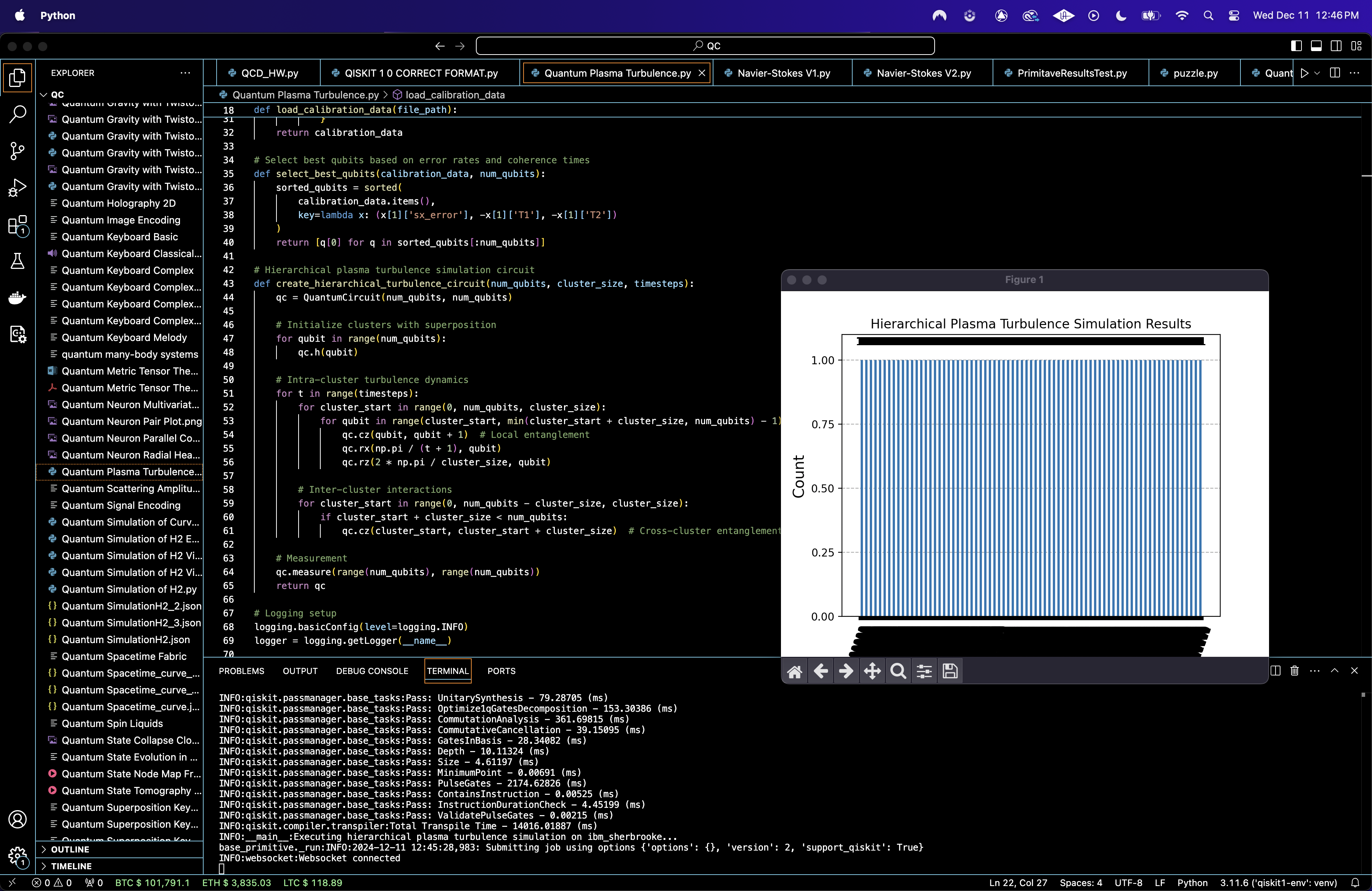
where x is a 127-bit string. This distribution is analyzed to extract patterns related to energy distribution and dissipation. The results are saved as a json and a histogram is visualized of shot counts.

Entropy = 13.0.
A high entropy value indicates that the quantum plasma turbulence simulation produced a state distribution with a high degree of randomness and complexity. This is consistent with turbulent systems, where energy dissipation leads to diverse state representations.
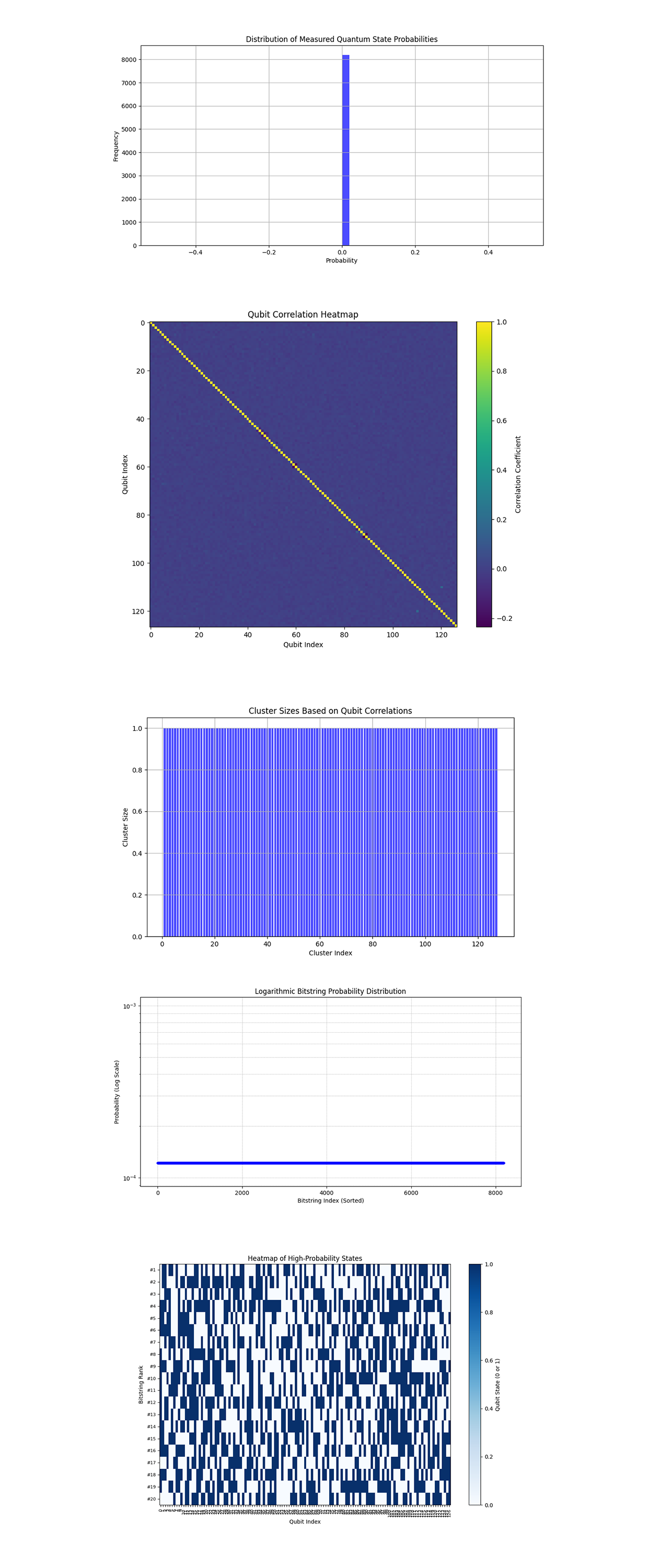
In the Distribution of Measured Quantum State Probabilities above (code below), the distribution is highly varied, with a majority of states concentrated near zero probability and a small number of states having measurable probabilities. This aligns with the physical intuition of turbulence, where energy dissipates unevenly, and only a few configurations dominate at any given time.
In the Qubit Correlation Heatmap above (code below), the heatmap shows strong self correlations (diagonal elements) as expected, but off diagonal correlations are weak with a few localized regions of slightly stronger interactions. The few pockets of slightly stronger correlations might represent localized energy transfers or transient interactions between qubits, potentially indicative of small scale structures within the turbulence.
In the Cluster Sizes Based on Qubit Correlations above (code below), all clusters have a size of 1, meaning there were no significant correlations between qubits strong enough to group them into larger clusters. This lack of clustering aligns with a highly chaotic turbulent system, where energy interactions are predominantly localized rather than forming larger coherent structures.
In the Logarithmic Bitstring Probability Distribution above (code below), the bitstring probabilities are highly sparse, with most probabilities near zero, except for a few slightly higher values. The sparsity reflects the localized energy dissipation that is a standard of turbulent systems.
In the Heatmap of High Probability States above (code below), the heatmap shows a varied configuration of qubit states for the top 20 bitstrings, with a mix of 0s and 1s. The diverse configurations support that quantum plasma turbulence results in highly varied but localized quantum states.

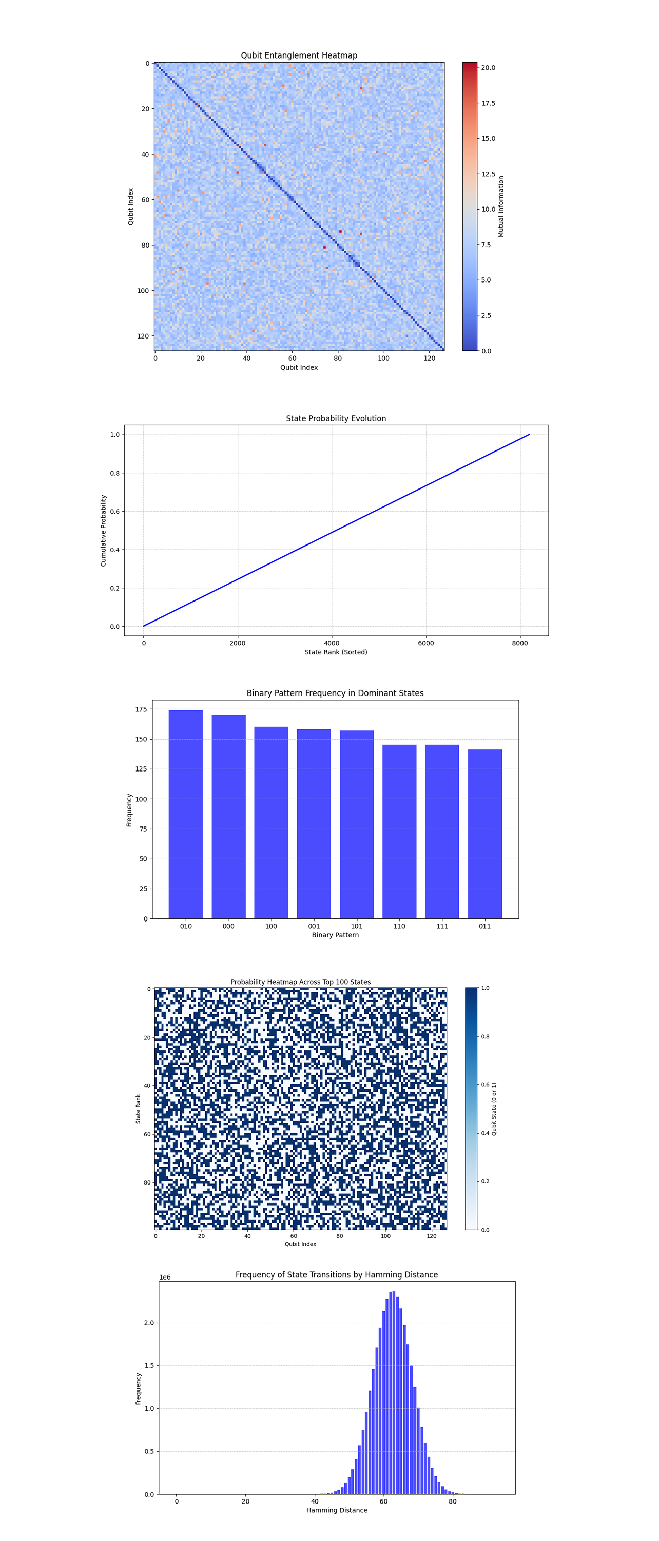
In the Qubit Entanglement Heatmap above (code below), the heatmap shows mutual information values between qubits, with most values close to zero. A few qubit pairs have relatively higher mutual information, indicating localized interactions. The predominantly low values suggest that the energy transfer between qubits is sparse, consistent with the sparse probability distribution observed earlier.
In the State Probability Evolution above (code below), the cumulative probability increases linearly with state rank, indicating a uniform contribution of states to the total probability.
In the Binary Pattern Frequency in Dominant States above (code below), Certain binary patterns (010, 000, 100) are more frequent in the top states. These repeating patterns represent quantum configurations that dominate under the simulated conditions. They might correspond to regions where energy interactions stabilize, forming recurring turbulence structures.
In the Probability Heatmap Across Top 100 States above (code below), the heatmap shows a high degree of randomness, with no discernible patterns in the qubit states of the top 100 most probable states.
In the Frequency of State Transitions (Hamming Distance) above (code below), the Hamming distances between states form a nearly Gaussian distribution, centered around half the number of qubits. This aligns with turbulence models, where the system explores states with widespread energy redistribution rather than small, incremental changes.

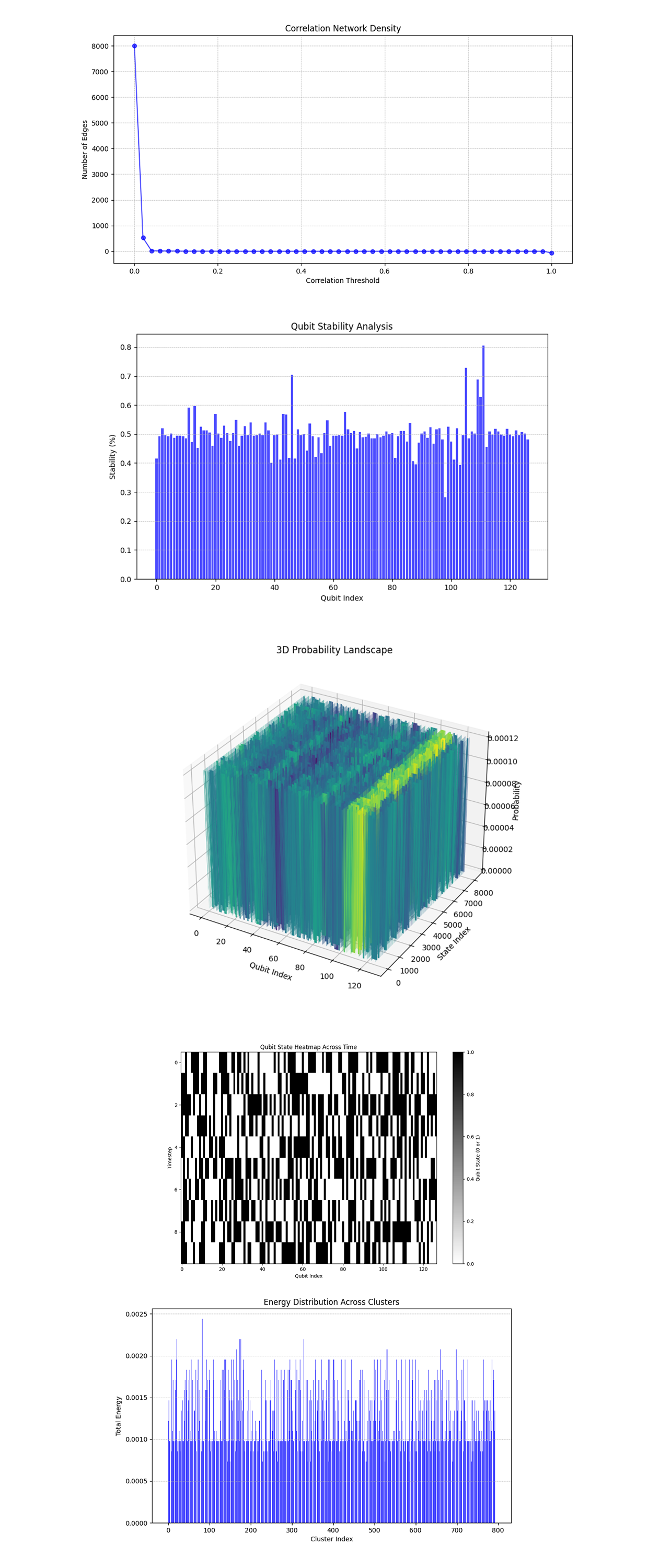
In the Correlation Network Density above (code below), the number of edges drops sharply as the correlation threshold increases, with almost all correlations disappearing by a threshold of 0.2. This rapid decline suggests weak correlations between qubits in the system, indicative of a highly chaotic and uncorrelated state.
In the Qubit Stability Analysis above (code below), the stability of qubits is uniform across the system, with most qubits having stability values around 0.5. A few qubits exhibit slightly higher stability values. The relatively uniform stability supports the model's depiction of turbulence as a system wide phenomenon without clear localization of stability.
In the 3D Probability Landscape above (code below), the 3D landscape reveals regions with slightly higher probabilities, but the overall distribution appears highly chaotic and distributed across states. The uniformity and lack of significant peaks suggest a turbulence model where energy dissipation is widespread and not strongly localized.
In the Qubit State Heatmap Across Time above (code below), the heatmap shows rapid, seemingly random state changes over time for most qubits.
In the Energy Distribution Across Clusters above (code below), the bar chart shows that energy (probabilities) is spread fairly evenly across clusters, with no single cluster dominating the energy landscape.
In the end, the quantum plasma turbulence experiment successfully simulated and analyzed energy dissipation and distribution in a chaotic quantum system. The simulation used qubit interactions to model turbulence dynamics, capturing the dynamic energy redistribution and localized interactions inherent to turbulent plasma systems.
Code:
Code (Main Circuit)
# Imports
import numpy as np
import json
import matplotlib.pyplot as plt
from qiskit import QuantumCircuit, transpile
from qiskit_ibm_runtime import QiskitRuntimeService, Session, SamplerV2
import csv
import logging
from collections import Counter
from qiskit.visualization import plot_histogram

# Parse calibration
def parse_field(field_str, parser=float, separator=";"):
    values = [parser(item.split(":")[1]) for item in field_str.split(separator) if ":" in item]
    return max(values) if values else 0.0

# Load calibration
def load_calibration_data(file_path):
    calibration_data = {}
    with open(file_path, 'r') as file:
        reader = csv.DictReader(file)
        for row in reader:
            qubit = int(row['Qubit'])
            calibration_data[qubit] = {
                'T1': float(row['T1 (us)'] or 0),
                'T2': float(row['T2 (us)'] or 0),
                'readout_error': float(row['Readout assignment error '] or 0),
                'sx_error': float(row['√x (sx) error '] or 0),
                'ecr_error': parse_field(row['ECR error '] or ""),
                'gate_time': parse_field(row['Gate time (ns)'] or "", parser=float)
            }
    return calibration_data

# Select best qubits based on error rates / coherence
def select_best_qubits(calibration_data, num_qubits):
    sorted_qubits = sorted(
        calibration_data.items(),
        key=lambda x: (x[1]['sx_error'], -x[1]['T1'], -x[1]['T2'])
    )
    return [q[0] for q in sorted_qubits[:num_qubits]]

# Hierarchical plasma turbulence
def create_hierarchical_turbulence_circuit(num_qubits, cluster_size, timesteps):
    qc = QuantumCircuit(num_qubits, num_qubits)

    # Initialize clusters with superposition
    for qubit in range(num_qubits):
        qc.h(qubit)

    # Intra-cluster turbulence dynamics
    for t in range(timesteps):
        for cluster_start in range(0, num_qubits, cluster_size):
            for qubit in range(cluster_start, min(cluster_start + cluster_size, num_qubits) - 1):
                qc. cz(qubit, qubit + 1)
                qc.rx(np.pi / (t + 1), qubit)
                qc.rz(2 * np.pi / cluster_size, qubit)

        # Inter-cluster interactions
        for cluster_start in range(0, num_qubits - cluster_size, cluster_size):
            if cluster_start + cluster_size < num_qubits:
                qc. cz(cluster_start, cluster_start + cluster_size)

    # Measurement
    qc.measure(range(num_qubits), range(num_qubits))
    return qc

# Logging
logging.basicConfig(level=logging. INFO)
logger = logging.getLogger(__name__)

# Calibration data
calibration_file = '/Users/Downloads/ibm_brisbane_calibrations_2024-12-11T20_28_38Z.csv'
calibration_data = load_calibration_data(calibration_file)

# Parameters
num_qubits = 127
cluster_size = 7
timesteps = 5
shots = 8192

# Select the best qubits
selected_qubits = select_best_qubits(calibration_data, num_qubits)

# IBMQ
service = QiskitRuntimeService(
    channel='ibm_quantum',
    instance='ibm-q/open/main',
    token='YOUR_IBMQ_API_O-`'
)

# Backend
backend_name = 'ibm_brisbane'
backend = service.backend(backend_name)

# Tanspile
qc = create_hierarchical_turbulence_circuit(num_qubits, cluster_size, timesteps)
transpiled_qc = transpile(qc, backend=backend, initial_layout=selected_qubits, optimization_level=3)

# Execute
with Session(service=service, backend=backend) as session:
    sampler = SamplerV2(session=session)
    logger. info("Executing hierarchical plasma turbulence simulation on ibm_sherbrooke...")
    job = sampler. run([transpiled_qc], shots=shots)
    job_result = job.result()

    # Results
    counts = dict(Counter(job_result._pub_results[0]['__value__']['data'].c.get_bitstrings()))
    results_data = {"counts": counts}
    output_file = '/Users/Documents/quantum_plasma_turbulence_results_0.json'
    with open(output_file, 'w') as f:
        json.dump(results_data, f, indent=4)

# Plot results
plot_histogram(counts)
plt.title("Hierarchical Plasma Turbulence Simulation Results")
plt. show()

logger. info("Experiment completed successfully.")

Visual Code 1
# Imports
import json
import matplotlib.pyplot as plt
import numpy as np

# Load results
file_path = '/Users/Documents/quantum_plasma_turbulence_results_0.json'
with open(file_path, 'r') as file:
    results_data = json.load(file)

# Extract counts
counts = results_data['counts']

# Normalize counts to probabilities
total_shots = sum(counts.values())
probabilities = {bitstring: count / total_shots for bitstring, count in counts.items()}

# Compute entropy of distribution
entropy = -sum(p * np.log2(p) for p in probabilities.values())

# Histogram of probabilities
prob_values = list(probabilities.values())
plt.figure(figsize=(12, 6))
plt.hist(prob_values, bins=50, color='blue', alpha=0.7)
plt.title('Distribution of Measured Quantum State Probabilities')
plt.xlabel('Probability')
plt.ylabel('Frequency')
plt.grid(True)
plt. show()

# Heatmap of qubit correlations
qubit_matrix = np.array([list(map(int, list(bitstring))) for bitstring in probabilities.keys()])
correlation_matrix = np.corrcoef(qubit_matrix.T)

plt.figure(figsize=(10, 8))
plt.imshow(correlation_matrix, cmap='viridis', aspect='auto')
plt.colorbar(label='Correlation Coefficient')
plt.title('Qubit Correlation Heatmap')
plt.xlabel('Qubit Index')
plt.ylabel('Qubit Index')
plt. show()

# Print entropy result
print(f"Entropy of the distribution: {entropy}")

Visual Code 2
# Imports
import json
import matplotlib.pyplot as plt
import numpy as np
import networkx as nx
from scipy.cluster.hierarchy import linkage, fcluster
from collections import Counter

# Load results
file_path = '/Users/Documents/quantum_plasma_turbulence_results_0.json'
with open(file_path, 'r') as file:
    results_data = json.load(file)

# Extract counts
counts = results_data['counts']

# Normalize counts to probabilities
total_shots = sum(counts.values())
probabilities = {bitstring: count / total_shots for bitstring, count in counts.items()}

# Convert bitstrings into a matrix of qubit states (0s and 1s) for correlation analysis
qubit_matrix = np.array([list(map(int, list(bitstring))) for bitstring in probabilities.keys()])
correlation_matrix = np.corrcoef(qubit_matrix.T)

# Cluster Analysis (Bar Chart)
Z = linkage(correlation_matrix, method='ward')
clusters = fcluster(Z, t=correlation_threshold, criterion='distance')
cluster_counts = Counter(clusters)

plt.figure(figsize=(10, 6))
plt. bar(cluster_counts.keys(), cluster_counts.values(), color='blue', alpha=0.7)
plt.title('Cluster Sizes Based on Qubit Correlations')
plt.xlabel('Cluster Index')
plt.ylabel('Cluster Size')
plt.grid(True)
plt. show()

# Bitstring Probability Distribution (Logarithmic)
sorted_probabilities = sorted(probabilities.values(), reverse=True)

plt.figure(figsize=(12, 6))
plt.plot(sorted_probabilities, marker='o', markersize=3, linestyle='-', color='blue', alpha=0.7)
plt.yscale('log')
plt.title('Logarithmic Bitstring Probability Distribution')
plt.xlabel('Bitstring Index (Sorted)')
plt.ylabel('Probability (Log Scale)')
plt.grid(True, which='both', linestyle='--', linewidth=0.5)
plt. show()

# Heatmap of High Probability States
top_bitstrings = sorted(probabilities.items(), key=lambda x: x[1], reverse=True)[:20]
top_states = np.array([list(map(int, list(bitstring))) for bitstring, _ in top_bitstrings])

plt.figure(figsize=(12, 8))
plt.imshow(top_states, cmap='Blues', aspect='auto', interpolation='none')
plt.colorbar(label='Qubit State (0 or 1)')
plt.title('Heatmap of High-Probability States')
plt.xlabel('Qubit Index')
plt.ylabel('Bitstring Rank')
plt.xticks(range(top_states.shape[1]), fontsize=8, rotation=90)
plt.yticks(range(len(top_bitstrings)), [f"#{i+1}" for i in range(len(top_bitstrings))], fontsize=8)
plt. show()

# Qubit Entanglement Heatmap
mutual_info_matrix = -np.log2(np.abs(correlation_matrix + 1e-9))  # Mutual information calculation
np.fill_diagonal(mutual_info_matrix, 0)

plt.figure(figsize=(10, 8))
plt.imshow(mutual_info_matrix, cmap='coolwarm', aspect='auto', interpolation='none')
plt.colorbar(label='Mutual Information')
plt.title('Qubit Entanglement Heatmap')
plt.xlabel('Qubit Index')
plt.ylabel('Qubit Index')
plt. show()

# State Probability Evolution
sorted_probs = sorted(probabilities.values(), reverse=True)
cumulative_probs = np.cumsum(sorted_probs)

plt.figure(figsize=(12, 6))
plt.plot(cumulative_probs, color='blue', linewidth=2)
plt.title('State Probability Evolution')
plt.xlabel('State Rank (Sorted)')
plt.ylabel('Cumulative Probability')
plt.grid(True, linestyle='--', linewidth=0.5)
plt. show()

# Binary Pattern Frequency
top_bitstrings = [bitstring for bitstring, _ in top_states]
substring_length = 3
substring_counts = Counter()

for bitstring in top_bitstrings:
for i in range(len(bitstring) - substring_length + 1):
substring = bitstring[i:i + substring_length]
substring_counts[substring] += 1

# Sort and plot top 10 substrings
most_common_substrings = substring_counts.most_common(10)
labels, values = zip(*most_common_substrings)

plt.figure(figsize=(10, 6))
plt. bar(labels, values, color='blue', alpha=0.7)
plt.title('Binary Pattern Frequency in Dominant States')
plt.xlabel('Binary Pattern')
plt.ylabel('Frequency')
plt.grid(axis='y', linestyle='--', linewidth=0.5)
plt. show()

# Probability Heatmap Across All States
sorted_indices = np.argsort(state_probs)[::-1]  # Sort states by probability (descending)
sorted_probs = np.array(state_probs)[sorted_indices]
heatmap_matrix = np.array([list(map(int, state_list[i])) for i in sorted_indices[:100]])  # Top 100 states

plt.figure(figsize=(12, 8))
plt.imshow(heatmap_matrix, cmap='Blues', aspect='auto', interpolation='none')
plt.colorbar(label='Qubit State (0 or 1)')
plt.title('Probability Heatmap Across Top 100 States')
plt.xlabel('Qubit Index')
plt.ylabel('State Rank')
plt. show()

# Frequency of State Transitions (Hamming Distance)
hamming_distances = []
for i, state1 in enumerate(state_list):
for state2 in state_list[i + 1:]:
hamming_distances.append(int(hamming(list(map(int, state1)), list(map(int, state2))) * len(state1)))

hamming_counts = np.bincount(hamming_distances)

plt.figure(figsize=(10, 6))
plt. bar(range(len(hamming_counts)), hamming_counts, color='blue', alpha=0.7)
plt.title('Frequency of State Transitions by Hamming Distance')
plt.xlabel('Hamming Distance')
plt.ylabel('Frequency')
plt.grid(axis='y', linestyle='--', linewidth=0.5)
plt. show()

# Correlation Network Density
correlation_matrix = np.corrcoef(qubit_matrix.T)
thresholds = np.linspace(0, 1, 50)
edge_counts = []

for threshold in thresholds:
edge_count = np.sum(np.abs(correlation_matrix) > threshold) - len(correlation_matrix)
edge_counts.append(edge_count / 2)

plt.figure(figsize=(12, 6))
plt.plot(thresholds, edge_counts, marker='o', color='blue', alpha=0.7)
plt.title('Correlation Network Density')
plt.xlabel('Correlation Threshold')
plt.ylabel('Number of Edges')
plt.grid(True, linestyle='--', linewidth=0.5)
plt. show()

# Qubit Stability Analysis
stability = (qubit_matrix == qubit_matrix[0]).mean(axis=0)

plt.figure(figsize=(10, 6))
plt. bar(range(len(stability)), stability, color='blue', alpha=0.7)
plt.title('Qubit Stability Analysis')
plt.xlabel('Qubit Index')
plt.ylabel('Stability (%)')
plt.grid(axis='y', linestyle='--', linewidth=0.5)
plt. show()

# 3D Probability Landscape
x = np.arange(qubit_matrix.shape[1])
y = np.arange(len(state_probs))
x, y = np.meshgrid(x, y)
z = np.array([state_probs[i] * qubit_matrix[i] for i in range(len(state_probs))])

fig = plt.figure(figsize=(12, 8))
ax = fig.add_subplot(111, projection='3d')
ax.plot_surface(x, y, z, cmap='viridis')
ax.set_title('3D Probability Landscape')
ax.set_xlabel('Qubit Index')
ax.set_ylabel('State Index')
ax.set_zlabel('Probability')
plt. show()

# Qubit State Heatmap
timesteps = 10

# Extract bitstrings and probabilities
bitstrings = list(results_data['counts'].keys())
bit_probs = list(results_data['counts'].values())
bit_probs = np.array(bit_probs) / sum(bit_probs)

# Sort bitstrings by their probabilities in descending order
sorted_indices = np.argsort(bit_probs)[::-1]  # Sort indices by probability (highest to lowest)
selected_bitstrings = [bitstrings[i] for i in sorted_indices[:timesteps]]

# Convert bitstrings into a binary matrix for heatmap visualization
state_evolution = np.array([list(map(int, bitstring)) for bitstring in selected_bitstrings])

# Plot heatmap
plt.figure(figsize=(12, 8))
plt.imshow(state_evolution, cmap='binary', aspect='auto', interpolation='none')
plt.colorbar(label='Qubit State (0 or 1)')
plt.title('Qubit State Heatmap Across Time')
plt.xlabel('Qubit Index')
plt.ylabel('Timestep')
plt. show()

# Energy Distribution Across Clusters
Z = linkage(qubit_matrix, method='ward')
clusters = fcluster(Z, t=10, criterion='distance')
cluster_counts = Counter(clusters)
cluster_energies = {cluster: 0 for cluster in cluster_counts.keys()}

# Calculate energy distribution across clusters
for state, cluster in zip(state_probs, clusters):
cluster_energies[cluster] += state

# Plot cluster energy distribution
plt.figure(figsize=(10, 6))
plt. bar(cluster_energies.keys(), cluster_energies.values(), color='blue', alpha=0.7)
plt.title('Energy Distribution Across Clusters')
plt.xlabel('Cluster Index')
plt.ylabel('Total Energy')
plt.grid(axis='y', linestyle='--', linewidth=0.5)
plt. show()

# End.
