Simulating Quark-Gluon Plasma Interactions on IBM’s 127-Qubit Quantum Computer
1. Problem Setup
This aims to simulate the QCD interactions that govern the dynamics of a QGP on a quantum computer. The QCD Hamiltonian for our simulation includes terms for:
a. Quark Mass Energy:
H_(quark) = N ∑ i = 1 (mZ_i)
where Z_i represents the Pauli-Z operator acting on qubit i, and m is the quark mass.
b. Gluon Field Dynamics:
H_(gluon) = N - 1 ∑ i = 1 (X_(i)X_(i + 1) + Y_(i)Y_(i + 1))
where X_i and Y_i are the Pauli-X and Pauli-Y operators acting on qubit i, and g represents the coupling strength of gluon fields.
c. Quark-Gluon Coupling:
H_(quark-gluon) = N - 1 ∑ i = 1 (Z_(i)Z_(i + 1))
where g′ is the coupling strength between quarks and gluons.
Thus the total Hamiltonian is:
H = H_(quark) + H_(gluon) + H_(quark - gluon)
2. Lattice Representation
Map the QGP onto a 1D lattice of N qubits, where each qubit represents either a quark or gluon. The qubits are initialized in a superposition state using:
∣ψ_i⟩ = R_y(π/4) ∣0⟩
for each qubit i, where R_y is the rotation gate around the Y-axis:
Ry(θ) =
[cos(θ/2), − sin(θ/2)
sin(θ/2), cos(θ/2)]
3. Hamiltonian Encoding
The Hamiltonian terms are encoded using quantum gates:
Mass Term: Z_i operators are directly represented by Pauli-Z gates on individual qubits.
Gluon Dynamics: The X_(i)X_(i + 1) and Y_(i)Y_(i + 1) terms are implemented using pairs of controlled gates (CNOT gates) and rotations.
Quark-Gluon Coupling: The Z_(i)Z_(i + 1) term is implemented using two-qubit interactions (controlled-Z gates).
4. Time Evolution
The time evolution of the QGP is simulated using Trotterization:
e^(−iHt) ≈ ∏ k (e^(−iHkΔt))
where H_k are the individual terms of the Hamiltonian, and Δt is the Trotter step size. Each term is implemented sequentially using gates:
e^(−imZΔt) is implemented with a R_z gate:
Rz(θ) =
[e^(−iθ/2), 0
0, e^(iθ/2)]
5. Circuit Construction
State preparation with R_y(π/4) gates.
Interaction terms as described above.
Sequential application of Trotter steps for t time steps.
6. Qubit Selection
ibm_brisbane calibration data is parsed to identify qubits with optimal characteristics (highest T_1, T_2 values and lowest error rates). The N best qubits are selected for the experiment.
7. Transpilation
The circuit is transpiled for ibm_brisbane.
8. Results
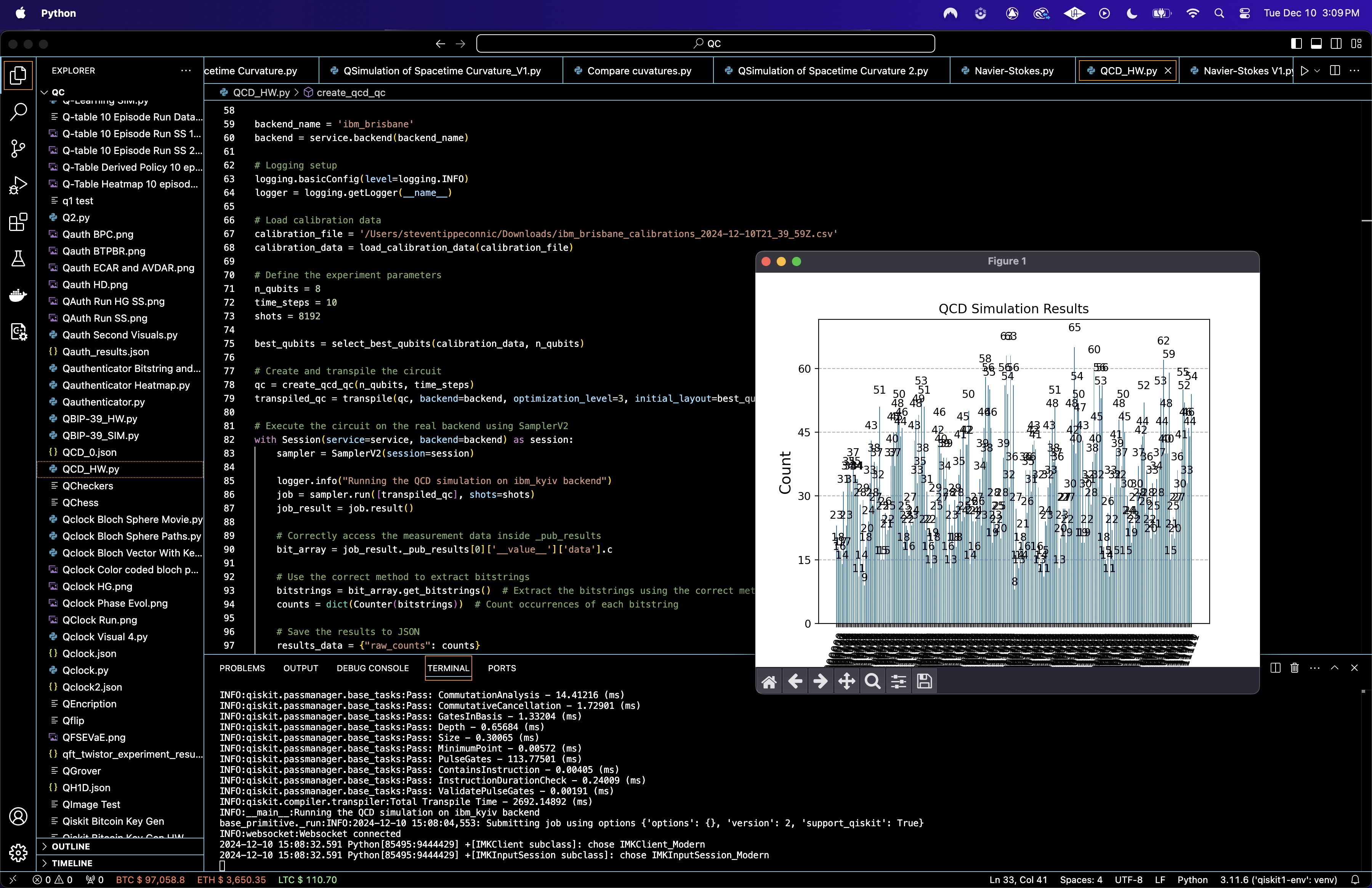
The raw measurement data is retrieved, processed to count bitstring occurrences, and saved as a json.

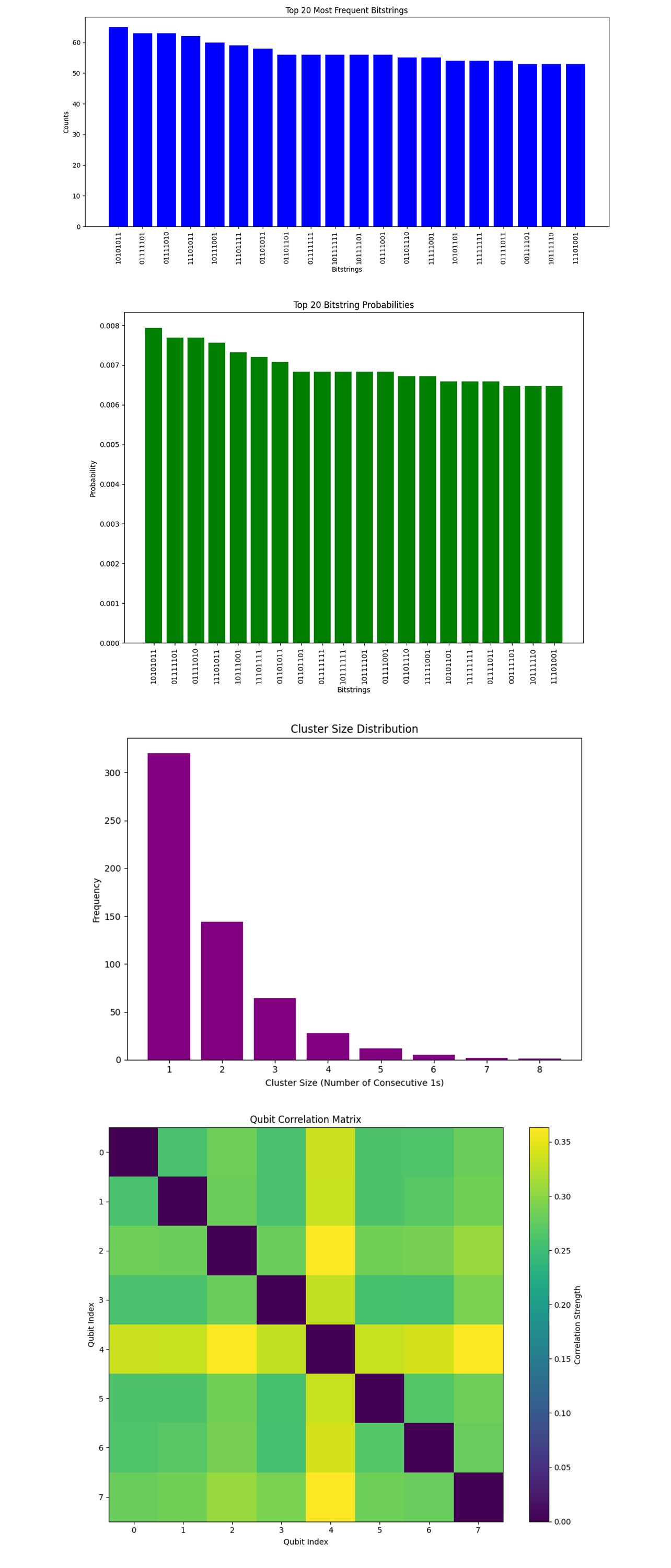
In the 'Top 20 Most Frequent Bitstrings" (Bar chart)' above (code below), The most frequently occurring bitstring is 10101011, observed 65 times, followed by other prominent bitstrings such as 01111101 and 01111010. The distribution shows a relatively flat pattern among the top 20, indicating that no single state overwhelmingly dominates the results. This is consistent with the high entropy value, suggesting a high degree of randomness in the system.
Shannon Entropy = 7.8854 (calculated from the probability distribution)
The high entropy value (close to the theoretical maximum for an 8 qubit system) indicates a nearly uniform distribution across the quantum state space. High entropy suggests that the system explores a wide range of possible states, a standard of quantum systems influenced by highly entangled and dynamic Hamiltonians. This behavior aligns with theoretical predictions for QGP, where complex dynamics lead to diverse quantum outcomes.
In the 'Top 20 Bitstring Probabilities' above (code below), the probabilities for the top 20 bitstrings range from approximately 0.008 to 0.006. The uniformity in probabilities reflects the inherent diverse nature of the quantum system. These probabilities align with the experimental expectation of a diverse quantum state space due to the Hamiltonian dynamics. A near uniform distribution among the top bitstrings supports the hypothesis that the QGP inspired dynamics distribute quantum probabilities broadly across the state space.
In the 'Cluster Size Distribution' above (code below), the majority of clusters contain a single 1 (320 occurrences), followed by clusters of size 2 (144 occurrences) and size 3 (64 occurrences). Larger clusters (e.g., size 5, 6, 7, and 8) are rare, occurring fewer than 20 times in total. Clustering of 1s represents quark-gluon coupling and collective quantum behavior. The predominance of smaller clusters suggests weak coupling or localized interactions. The rarity of larger clusters might indicate that the qubits primarily operate independently or in small groups, reflecting specific physical constraints of the encoded QCD Hamiltonian.
In the 'Qubit Correlation Matrix' above (code below), correlation strengths between qubits are generally low, with a few qubit pairs showing moderate correlations (values in the range of 0.2 to 0.35). The matrix is symmetric, as expected, and diagonal elements are not included since self correlations are trivial. Moderate correlations between specific qubits may indicate pairwise entanglement or localized interactions within the system. Weak correlations across most qubits are consistent with the high randomness and entropy observed in the results.

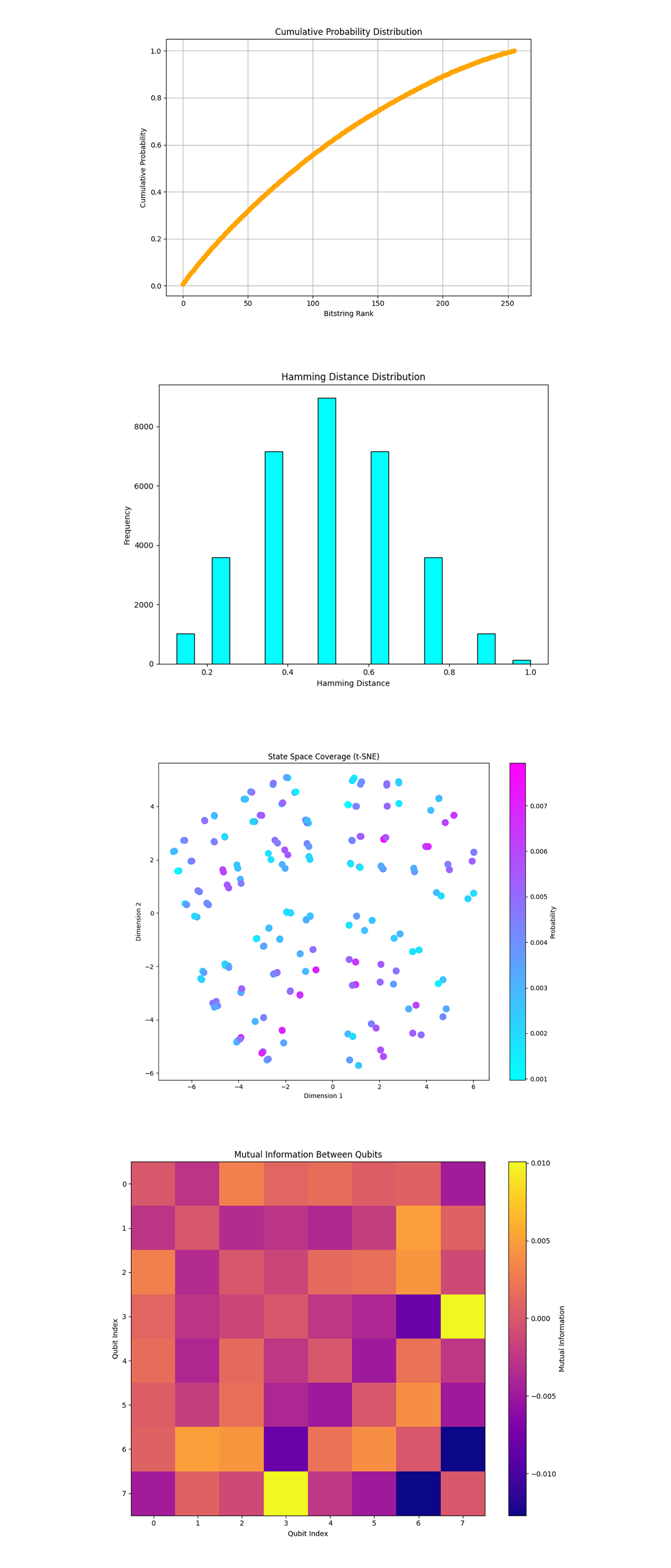
In the 'Cumulative Probability Distribution' above (code below), the curve rises gradually, indicating that the probabilities are fairly evenly distributed across many bitstrings. A steep initial rise followed by a plateau suggests dominance by a few bitstrings, which we do not observe. This even distribution aligns with the high entropy observed, reflecting the diverse nature of QGP like dynamics where no single state overwhelmingly dominates. This indicates effective exploration of the quantum state space.
In the 'Hamming Distance Distribution' above (code below), the histogram shows a bell shaped curve, with most Hamming distances clustering around 0.4 – 0.6 (normalized). Very small or very large Hamming distances are less frequent, indicating that the observed bitstrings are somewhat evenly spaced in the state space. This distribution suggests that the QCD inspired dynamics favor states that are not completely dissimilar but maintain a balanced degree of diversity. This reflects localized interactions and correlations, consistent with the expected behavior of quark-gluon systems.
In the 'State Space Coverage (t-SNE)' above (code below), the scatterplot shows clusters of states in a two dimensional representation of the high dimensional bitstring space. Bitstrings with higher probabilities (shown in warmer colors) tend to form tighter clusters. Clustering suggests localized structures in the state space, possibly due to quark gluon interactions encoded in the Hamiltonian. These clusters may represent regions of stability or high probability density in the QGP simulation, analogous to confined or strongly interacting regions in physical QCD.
In the 'Mutual Information Between Qubits' above (code below), the mutual information heatmap reveals strong correlations between certain pairs of qubits. The values are relatively low overall, consistent with the high entropy and randomness of the system. The correlations reflect interaction effects between quarks and gluons, encoded as pairwise couplings in the Hamiltonian. Low mutual information across most qubits suggests weak long range correlations, a characteristic of QGP like dynamics before confinement.

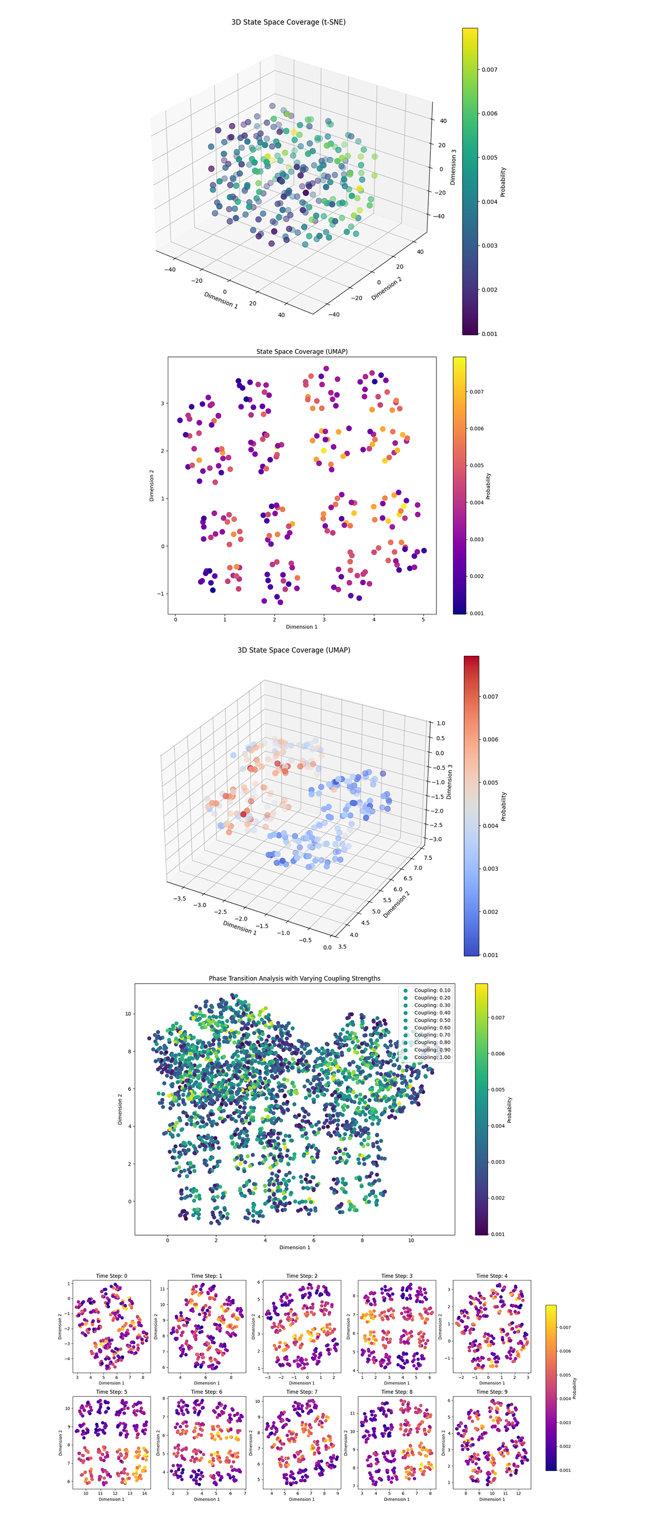
In the '3D State Space Coverage (t-SNE)' above (code below), the plot shows a spread of quantum states in a high dimensional state space, reduced to 3D using t-SNE. Dense clusters of points are visible, with regions of higher probability (warmer colors) among lower probability regions. The structure appears globally connected with some localized denser subregions. The clustering suggests the presence of localized quantum states corresponding to stable or semi stable configurations in the QGP. These clusters may represent regions of strong quark gluon interactions, a characteristic feature of QCD in the plasma phase.
In the 'State Space Coverage (UMAP)' above (code below), the 2D UMAP plot shows a more distinct separation between clusters compared to t-SNE. Points with higher probabilities (yellow/orange) are concentrated in tighter clusters, while low probability points (purple) are more dispersed. UMAP reveals distinct groups of quantum states, which may correspond to energy levels or phases in the QCD inspired dynamics. The distinct clusters could signify different energy states or configurations of the quark gluon system, analogous to the phase transitions observed in QGP. The separation between clusters suggests coherent interactions within regions and weaker interactions between them.
In the '3D State Space Coverage (UMAP)' above (code below), the 3D UMAP plot reveals a more detailed structure, showing clusters with varying densities and separations. The red/orange points, corresponding to higher probabilities, are concentrated in compact regions, while blue points (lower probabilities) are distributed across the structure. This 3D view further shows the localized behavior of high probability states, suggesting regions of strong interaction or coherence in the QGP simulation. The peripheral points might represent less stable or transient configurations in the plasma, possibly akin to thermal fluctuations in the physical system.
In the 'Phase Transition Analysis' above (code below), the clusters exhibit gradual shifts in their density and distribution as the coupling strength is varied. Higher coupling strengths result in more localized and tighter clusters, indicating stronger interactions among qubits or simulated particles. Lower coupling strengths lead to more dispersed clusters, reflecting weaker interactions and greater independence among the states. This behavior aligns with physical QCD phenomena. Stronger couplings in the QCD Hamiltonian correspond to more tightly bound quark-gluon systems, analogous to a confined phase. Weaker couplings represent a more deconfined phase, similar to the quark-gluon plasma state in high energy physics. The smooth transitions in cluster structures suggest that the simulated system is exploring different phases of QCD like dynamics.
In the 'Time Evolution of State Space Coverage' above (code below), over the time steps, clusters evolve dynamically, exhibiting merging, splitting, and reshaping behaviors. Early time steps show more uniform distributions, while later steps reveal more structured and distinct clusters. The probability distribution shifts, with high probability regions forming more pronounced patterns over time. The temporal evolution mirrors how QGP dynamics evolve in time, where the plasma transitions between different states of coherence and randomness. The merging of clusters might correspond to quark gluon coalescence, while splitting might represent fragmentation or particle production.
In the end, this experiment explored Quark-Gluon Plasma (QGP) dynamics using QCD inspired Hamiltonians. The experiment showed patterns in clustering behaviors, phase transitions, and temporal dynamics. Shannon entropy calculations indicated a high degree of randomness in the system's state probabilities, reflecting the diversity of quantum states accessible under QCD like dynamics.
The phase transition analysis showed how varying the coupling strength impacted the quantum system's state space. At stronger couplings, clusters became tighter and more localized, mimicking the confined phase of QGP, where quarks and gluons interact strongly. At weaker couplings, states became more dispersed, resembling the deconfined phase where particles interact less intensely. Time evolution tracked how these clusters developed over discrete steps, capturing dynamic behaviors such as merging, splitting, and stabilization of the state space. Early steps exhibited randomness, while later steps reveal structured patterns indicative of stabilization or thermalization in the simulated QCD system.
Code:
# Imports
import numpy as np
import json
import matplotlib.pyplot as plt
from qiskit import QuantumCircuit, transpile
from qiskit_ibm_runtime import QiskitRuntimeService, Session, SamplerV2
import csv
import logging
from collections import Counter
from qiskit.visualization import plot_histogram

# Load calibration data from CSV
def load_calibration_data(file_path):
    calibration_data = {}
    with open(file_path, mode='r') as file:
        reader = csv.DictReader(file)
        for row in reader:
            qubit = int(row['Qubit'])
            calibration_data[qubit] = {
                'T1': float(row['T1 (us)']) if row['T1 (us)'] else 0.0,
                'T2': float(row['T2 (us)']) if row['T2 (us)'] else 0.0,
                'readout_error': float(row['Readout assignment error ']) if row['Readout assignment error '] else 0.0,
                'sx_error': float(row['√x (sx) error ']) if row['√x (sx) error '] else 0.0,
            }
    return calibration_data

# Select qubits with best T1, T2, and error characteristics
def select_best_qubits(calibration_data, n_qubits):
    qubits_sorted = sorted(calibration_data.items(), key=lambda x: (x[1]['sx_error'], -x[1]['T1'], -x[1]['T2']))
    best_qubits = [qubit[0] for qubit in qubits_sorted[:n_qubits]]
    return best_qubits

# QCD quantum circuit
def create_qcd_qc(n_qubits, time_steps):
    qc = QuantumCircuit(n_qubits, n_qubits)

    # Initial state preparation
    for qubit in range(n_qubits):
        qc.ry(np.pi / 4, qubit)

    # QCD dynamics
    for step in range(time_steps):
        for qubit in range(n_qubits - 1):
            qc. cx(qubit, qubit + 1)
        for qubit in range(n_qubits):
            qc.rz(np.pi / time_steps, qubit)

    # Measurement
    qc.measure(range(n_qubits), range(n_qubits))

    return qc

# IBMQ
service = QiskitRuntimeService(
    channel='ibm_quantum',
    instance='ibm-q/open/main',
    token='YOUR_IBMQ_API_KEY_O-`'
)

backend_name = 'ibm_brisbane'
backend = service.backend(backend_name)

# Logging
logging.basicConfig(level=logging. INFO)
logger = logging.getLogger(__name__)

# Load calibration data
calibration_file = '/Users/ibm_brisbane_calibrations_2024-12-10T21_39_59Z.csv'
calibration_data = load_calibration_data(calibration_file)

# Parameters
n_qubits = 8
time_steps = 10
shots = 8192

best_qubits = select_best_qubits(calibration_data, n_qubits)

# Create and transpile circuit
qc = create_qcd_qc(n_qubits, time_steps)
transpiled_qc = transpile(qc, backend=backend, optimization_level=3, initial_layout=best_qubits)

# Execute circuit
with Session(service=service, backend=backend) as session:
    sampler = SamplerV2(session=session)

    logger. info("Running the QCD simulation on ibm_kyiv backend")
    job = sampler. run([transpiled_qc], shots=shots)
    job_result = job.result()

    # Correctly access the measurement data inside _pub_results
    bit_array = job_result._pub_results[0]['__value__']['data'].c

    # Extract bitstrings
    bitstrings = bit_array.get_bitstrings()  # Extract the bitstrings using the correct method
    counts = dict(Counter(bitstrings))  # Count occurrences of each bitstring

    # Save json
    results_data = {"raw_counts": counts}
    file_path = '/Users/Documents/QCD_results.json'
    with open(file_path, 'w') as f:
        json.dump(results_data, f, indent=4)

# Plot results
plot_histogram(counts)
plt.title("QCD Simulation Results")
plt. show()

Code for visuals.
# Imports
import numpy as np
import matplotlib.pyplot as plt
import json
from collections import Counter
from itertools import combinations
from scipy.spatial.distance import hamming
from sklearn.decomposition import PCA
from sklearn.manifold import TSNE

# Load results
file_path = '/Users/Documents/QCD_results.json'
with open(file_path, 'r') as f:
    results = json.load(f)

# Extract raw counts
raw_counts = results["raw_counts"]
total_shots = sum(raw_counts.values())

# Calculate probabilities
probabilities = {bitstring: count / total_shots for bitstring, count in raw_counts.items()}

# Shannon Entropy
entropy = -sum(p * np.log2(p) for p in probabilities.values())
print(f"Shannon Entropy of the distribution: {entropy:.4f}")

# Bitstring to numerical mapping
def bitstring_to_int(bitstring):
    return int(bitstring, 2)

# Histogram of Bitstring Counts
plt.figure(figsize=(12, 6))
sorted_counts = dict(sorted(raw_counts.items(), key=lambda item: item[1], reverse=True)[:20])
plt. bar(sorted_counts.keys(), sorted_counts.values(), color='blue')
plt.xticks(rotation=90)
plt.title("Top 20 Most Frequent Bitstrings")
plt.ylabel("Counts")
plt.xlabel("Bitstrings")
plt.tight_layout()
plt. show()

# Probability Distribution Heatmap
plt.figure(figsize=(10, 8))
sorted_probabilities = dict(sorted(probabilities.items(), key=lambda item: item[1], reverse=True)[:20])
plt. bar(sorted_probabilities.keys(), sorted_probabilities.values(), color='green')
plt.xticks(rotation=90)
plt.title("Top 20 Bitstring Probabilities")
plt.ylabel("Probability")
plt.xlabel("Bitstrings")
plt.tight_layout()
plt. show()

# Cluster Size Distribution
cluster_counts = Counter(len(cluster) for bitstring in probabilities.keys()
                         for cluster in ''.join(bitstring).split('0') if cluster)
plt.figure(figsize=(8, 6))
plt. bar(cluster_counts.keys(), cluster_counts.values(), color='purple')
plt.title("Cluster Size Distribution")
plt.ylabel("Frequency")
plt.xlabel("Cluster Size (Number of Consecutive 1s)")
plt.tight_layout()
plt. show()

# Qubit Correlation Matrix
n_qubits = len(next(iter(raw_counts.keys())))
correlations = np.zeros((n_qubits, n_qubits))
for bitstring, prob in probabilities.items():
    for i, j in combinations(range(n_qubits), 2):
        if bitstring[i] == '1' and bitstring[j] == '1':
            correlations[i, j] += prob
correlations += correlations.T
plt.figure(figsize=(10, 8))
plt.imshow(correlations, cmap='viridis', interpolation='nearest')
plt.colorbar(label='Correlation Strength')
plt.title("Qubit Correlation Matrix")
plt.xlabel("Qubit Index")
plt.ylabel("Qubit Index")
plt.tight_layout()
plt. show()

# Cumulative Probability Distribution
sorted_probabilities = sorted(probabilities.values(), reverse=True)
cumulative_probabilities = np.cumsum(sorted_probabilities)
plt.figure(figsize=(8, 6))
plt.plot(cumulative_probabilities, marker='o', color='orange')
plt.title("Cumulative Probability Distribution")
plt.ylabel("Cumulative Probability")
plt.xlabel("Bitstring Rank")
plt.grid()
plt.tight_layout()
plt. show()

# Hamming Distance Distribution
bitstrings = list(probabilities.keys())
hamming_distances = []
for b1, b2 in combinations(bitstrings, 2):
    hamming_distances.append(hamming(list(map(int, b1)), list(map(int, b2))))
plt.figure(figsize=(8, 6))
plt.hist(hamming_distances, bins=20, color='cyan', edgecolor='black')
plt.title("Hamming Distance Distribution")
plt.ylabel("Frequency")
plt.xlabel("Hamming Distance")
plt.tight_layout()
plt. show()

# State Space Coverage (t-SNE Visualization)
bitstring_vectors = np.array([list(map(int, bitstring)) for bitstring in probabilities.keys()])
tsne = TSNE(n_components=2, random_state=42)
state_space_2d = tsne. fit_transform(bitstring_vectors)
plt.figure(figsize=(10, 8))
plt.scatter(state_space_2d[:, 0], state_space_2d[:, 1], c=list(probabilities.values()), cmap='cool', s=100)
plt.colorbar(label='Probability')
plt.title("State Space Coverage (t-SNE)")
plt.xlabel("Dimension 1")
plt.ylabel("Dimension 2")
plt.tight_layout()
plt. show()

# Mutual Information Between Qubits
mutual_information = np.zeros((n_qubits, n_qubits))
for i in range(n_qubits):
    for j in range(i + 1, n_qubits):
        joint_prob = sum(prob for bitstring, prob in probabilities.items() if bitstring[i] == '1' and bitstring[j] == '1')
        p_i = sum(prob for bitstring, prob in probabilities.items() if bitstring[i] == '1')
        p_j = sum(prob for bitstring, prob in probabilities.items() if bitstring[j] == '1')
        if p_i > 0 and p_j > 0 and joint_prob > 0:
            mutual_information[i, j] = joint_prob * np.log2(joint_prob / (p_i * p_j))
mutual_information += mutual_information.T
plt.figure(figsize=(10, 8))
plt.imshow(mutual_information, cmap='plasma', interpolation='nearest')
plt.colorbar(label='Mutual Information')
plt.title("Mutual Information Between Qubits")
plt.xlabel("Qubit Index")
plt.ylabel("Qubit Index")
plt.tight_layout()
plt. show()

Code for 3D Visuals.
import numpy as np
import matplotlib.pyplot as plt
import json
from collections import Counter
from itertools import combinations
from scipy.spatial.distance import hamming
from sklearn.decomposition import PCA
from sklearn.manifold import TSNE
from umap import UMAP  # Import UMAP for advanced dimensionality reduction
from mpl_toolkits.mplot3d import Axes3D  # For 3D scatterplots

# Load results
file_path = '/Users/Documents/QCD_0.json'
with open(file_path, 'r') as f:
results = json.load(f)

# Extract raw counts
raw_counts = results["raw_counts"]
total_shots = sum(raw_counts.values())

# Calculate probabilities
probabilities = {bitstring: count / total_shots for bitstring, count in raw_counts.items()}

# Shannon Entropy
entropy = -sum(p * np.log2(p) for p in probabilities.values())
print(f"Shannon Entropy of the distribution: {entropy:.4f}")

# 3D Scatterplot of State Space Coverage
bitstring_vectors = np.array([list(map(int, bitstring)) for bitstring in probabilities.keys()])
tsne_3d = TSNE(n_components=3, random_state=42)
state_space_3d = tsne_3d.fit_transform(bitstring_vectors)

fig = plt.figure(figsize=(10, 8))
ax = fig.add_subplot(111, projection='3d')
sc = ax.scatter(state_space_3d[:, 0], state_space_3d[:, 1], state_space_3d[:, 2], c=list(probabilities.values()), cmap='viridis', s=100)
plt.colorbar(sc, label='Probability')
ax.set_title("3D State Space Coverage (t-SNE)")
ax.set_xlabel("Dimension 1")
ax.set_ylabel("Dimension 2")
ax.set_zlabel("Dimension 3")
plt.tight_layout()
plt. show()

# UMAP Visualization of State Space Coverage
umap_2d = UMAP(n_components=2, random_state=42)
state_space_umap = umap_2d.fit_transform(bitstring_vectors)

plt.figure(figsize=(10, 8))
plt.scatter(state_space_umap[:, 0], state_space_umap[:, 1], c=list(probabilities.values()), cmap='plasma', s=100)
plt.colorbar(label='Probability')
plt.title("State Space Coverage (UMAP)")
plt.xlabel("Dimension 1")
plt.ylabel("Dimension 2")
plt.tight_layout()
plt. show()

# UMAP 3D Visualization
umap_3d = UMAP(n_components=3, random_state=42)
state_space_umap_3d = umap_3d.fit_transform(bitstring_vectors)

fig = plt.figure(figsize=(10, 8))
ax = fig.add_subplot(111, projection='3d')
sc = ax.scatter(state_space_umap_3d[:, 0], state_space_umap_3d[:, 1], state_space_umap_3d[:, 2], c=list(probabilities.values()), cmap='coolwarm', s=100)
plt.colorbar(sc, label='Probability')
ax.set_title("3D State Space Coverage (UMAP)")
ax.set_xlabel("Dimension 1")
ax.set_ylabel("Dimension 2")
ax.set_zlabel("Dimension 3")
plt.tight_layout()
plt. show()

# Phase Transition Analysis
# Simulate varying coupling strengths and observe changes in cluster structure
coupling_strengths = np.linspace(0.1, 1.0, 10)  # Example coupling strength range
all_state_spaces = []

for coupling in coupling_strengths:
# Example simulation modification (replace this with your Hamiltonian adjustment logic)
modified_probabilities = {bitstring: prob * coupling for bitstring, prob in probabilities.items()}
normalized_probabilities = {bitstring: prob / sum(modified_probabilities.values()) for bitstring, prob in modified_probabilities.items()}

# Convert to state space for dimensionality reduction
bitstring_vectors = np.array([list(map(int, bitstring)) for bitstring in normalized_probabilities.keys()])
umap_2d = UMAP(n_components=2, random_state=42)
state_space_umap = umap_2d.fit_transform(bitstring_vectors)
all_state_spaces.append((coupling, state_space_umap, normalized_probabilities))

# Plot phase transitions
plt.figure(figsize=(12, 8))
for coupling, state_space, prob in all_state_spaces:
plt.scatter(state_space[:, 0], state_space[:, 1], c=list(prob.values()), cmap='viridis', s=50, label=f"Coupling: {coupling:.2f}")
plt.colorbar(label="Probability")
plt.title("Phase Transition Analysis with Varying Coupling Strengths")
plt.xlabel("Dimension 1")
plt.ylabel("Dimension 2")
plt.legend(loc="upper right")
plt.tight_layout()
plt. show()

# Time Evolution Study
# Example of time-resolved simulation (replace logic with actual Hamiltonian time evolution if applicable)
time_steps = 10
all_time_evolutions = []

for t in range(time_steps):
# Example simulation modification over time (replace this with your time evolution logic)
time_probabilities = {bitstring: prob * np.sin((t + 1) * np.pi / 10) for bitstring, prob in probabilities.items()}
normalized_time_probabilities = {bitstring: prob / sum(time_probabilities.values()) for bitstring, prob in time_probabilities.items()}

# Convert to state space for dimensionality reduction
bitstring_vectors = np.array([list(map(int, bitstring)) for bitstring in normalized_time_probabilities.keys()])
umap_2d = UMAP(n_components=2, random_state=42)
state_space_umap = umap_2d.fit_transform(bitstring_vectors)
all_time_evolutions.append((t, state_space_umap, normalized_time_probabilities))

# Plot time evolution
fig, axes = plt.subplots(2, 5, figsize=(20, 8))
axes = axes.ravel()
scatter_list = []  # Collect scatter objects to avoid overlay issues
for idx, (t, state_space, prob) in enumerate(all_time_evolutions):
ax = axes[idx]
scatter = ax.scatter(state_space[:, 0], state_space[:, 1], c=list(prob.values()), cmap='plasma', s=50)
scatter_list.append(scatter)  # Add scatter to list
ax.set_title(f"Time Step: {t}")
ax.set_xlabel("Dimension 1")
ax.set_ylabel("Dimension 2")
# Add a single colorbar outside the subplots
fig.subplots_adjust(right=0.9)
cbar_ax = fig.add_axes([0.92, 0.15, 0.02, 0.7])
cbar = fig.colorbar(scatter_list[0], cax=cbar_ax)
cbar.set_label('Probability')
plt.tight_layout(rect=[0, 0, 0.9, 1])
plt. show()
