Exploring the Navier-Stokes Equations Using Carleman Linearization on IBM’s 127-Qubit Quantum Computer

This experiment using qiskit explores the Navier-Stokes equations, which describe fluid dynamics, using Carleman linearization. This quantum circuit aims to explore the utility of quantum computing in solving nonlinear differential equations. The experiment runs on @IBM's ibm_brisbane 127-qubit quantum computer. The circuit encodes the nonlinear behavior of fluid flow into a quantum system, using quantum entanglement and superposition to handle the linearized approximation of these equations.
The results showed that the quantum system converged to a small number of stable quantum states. These states represent stable or low-energy configurations of the fluid system. In classical fluid dynamics, this would be akin to the fluid reaching an equilibrium or stable flow pattern. Thus, we observed the emergence of dominant, stable fluid configurations.

1. The Navier-Stokes Equations
The Navier-Stokes equations describe the motion of fluid substances such as liquids and gases. The general form is given by:
ρ((∂u/∂t) + (u⋅∇)u) = −∇p + μ∇²u + f
Where:
u = (u, v, w) is the velocity field.
ρ is the fluid density.
p is the pressure field.
μ is the dynamic viscosity.
f represents external forces acting on the fluid.
For this experiment, we focus on the Carleman linearization approach, which allows us to approximate these nonlinear equations with a set of linear equations.

2. Carleman Linearization
Carleman linearization approximates a nonlinear system by embedding it into a higher-dimensional linear space. The Navier-Stokes equations, being nonlinear due to the (u⋅∇)u term, can be transformed into a linear form by introducing auxiliary variables that capture higher order interactions.
In mathematical terms, we approximate the velocity field evolution using a linear system of equations by truncating higher-order terms. Let’s denote the approximated linear system as:

x_(n + 1) = Ax_n + B
Where A is a matrix capturing the linearized evolution of the system, and B is a vector that captures constant or external forces. In quantum computing, this evolution is mapped onto a quantum circuit where the state evolves step by step according to these linearized dynamics.

3. Quantum Circuit Design
To simulate the Navier-Stokes dynamics on a quantum computer, we design a quantum circuit where each qubit represents a component of the velocity field. The quantum gates simulate the linearized evolution over discrete time steps. The circuit includes:
Initialization: Each qubit is initialized to a superposition state using the R_y gate, which encodes initial fluid velocities.
Ry(θ) =
((cos(θ/2), −sin(θ/2)
(sin(θ/2), cos(θ/2))
Time evolution of the velocity field is simulated using rotation gates R_z and entangling gates CX. The R_z gate rotates the phase of the qubit to capture the time evolution of fluid velocity:
Rz(θ) =
((e^(−iθ/2), 0)
(0, e^(iθ/2))
The CX (CNOT) gates simulate interactions between neighboring fluid particles (qubits), capturing the coupling between different velocity components due to the nonlinear term in Navier-Stokes.

4. Noise-Adaptive Transpilation
The calibration file for ibm_brisbane includes information like T1, T2 times, gate errors, and readout errors. This data is used to select the qubits with the best performance characteristics.
The circuit is transpiled using the Sabre routing algorithm, which minimizes the impact of noise by dynamically choosing the most reliable qubits and gates based on their error rates.

5. Running the Experiment
The quantum circuit is executed on IBM’s ibm_brisbane using SamplerV2 to simulate the fluid dynamics over time. The circuit is run with 8192 shots.

6. Result Collection
The quantum hardware returns a set of bitstrings representing the fluid velocities at different time steps.

7. Post-Processing and Visualization
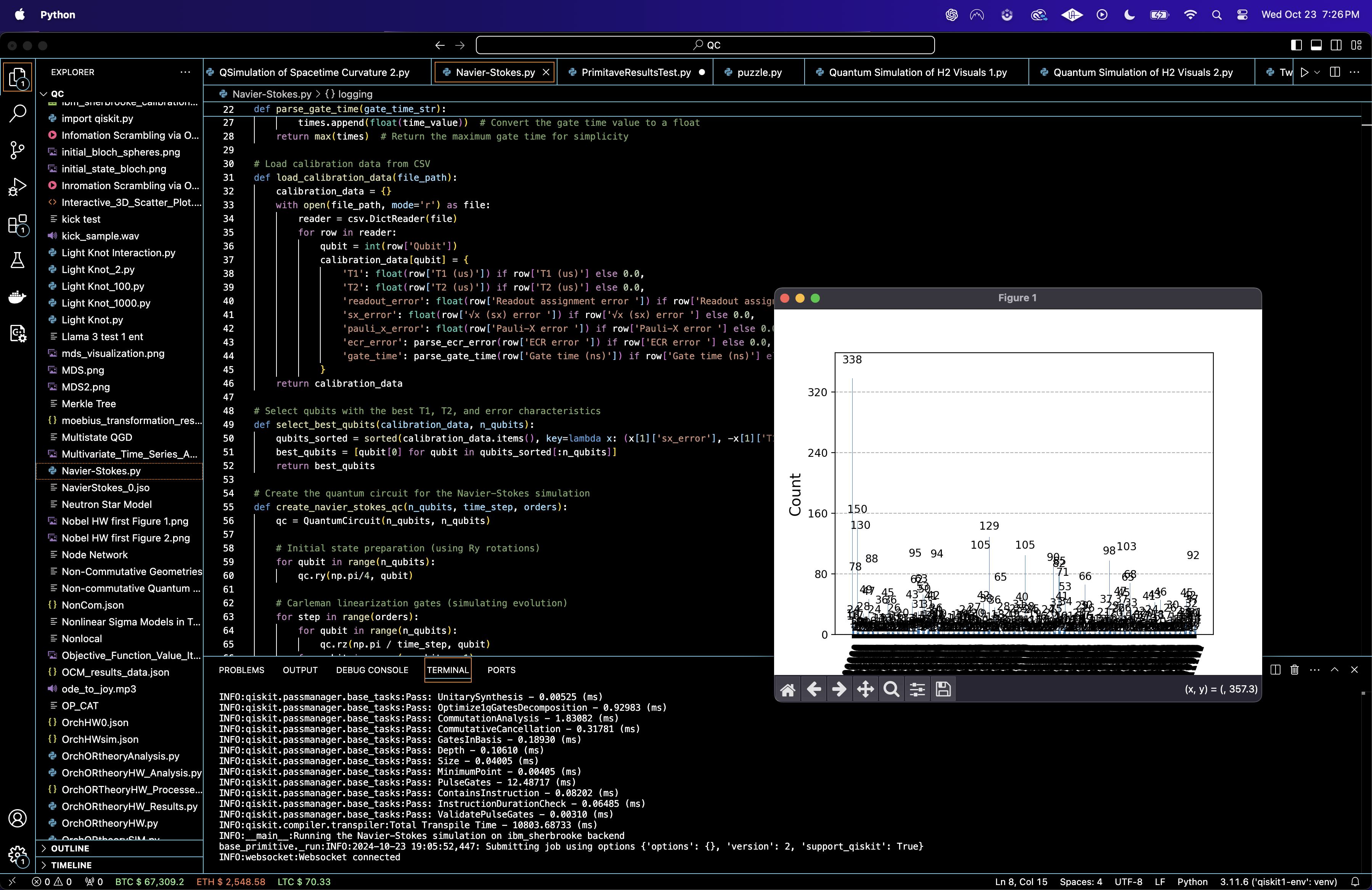
The counts are saved in a JSON. A histogram of the results is plotted.

Results:

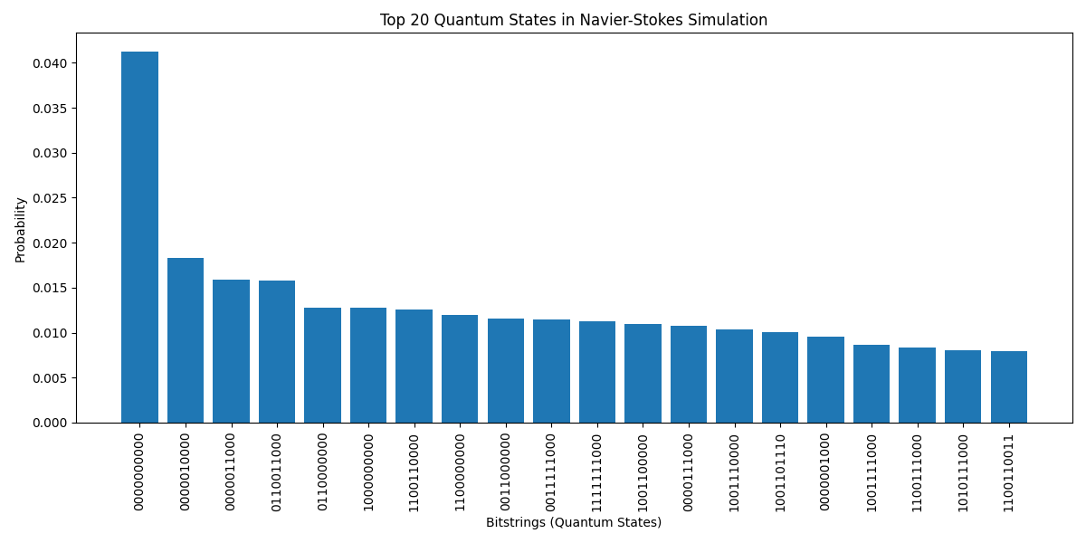
The bar chart above (code below) reveals that a single quantum state ("0000000000") dominates the results with a probability of over 4%. This suggests that this particular configuration, corresponding to a low-energy or stable configuration in the Navier-Stokes system, is highly favored. The other quantum states exhibit probabilities between 1% and 2%, reflecting a mixture of possible fluid configurations but with lower likelihoods.
The results showed that the quantum system, simulating the linearized Navier-Stokes equations using Carleman linearization, converged to a small number of stable quantum states. These states represent stable or low-energy configurations of the fluid system. In classical fluid dynamics, this would be akin to the fluid reaching an equilibrium or stable flow pattern. Thus, we observed the emergence of dominant, stable fluid configurations.
A significant portion of the quantum states had very low probabilities, suggesting that more complex or turbulent fluid configurations are rare but still possible. In classical terms, these rare states may correspond to more intricate flow patterns, including localized turbulence or transient phenomena. The low probability of these states indicates that the system mostly avoids these complex dynamics but occasionally exhibits them.

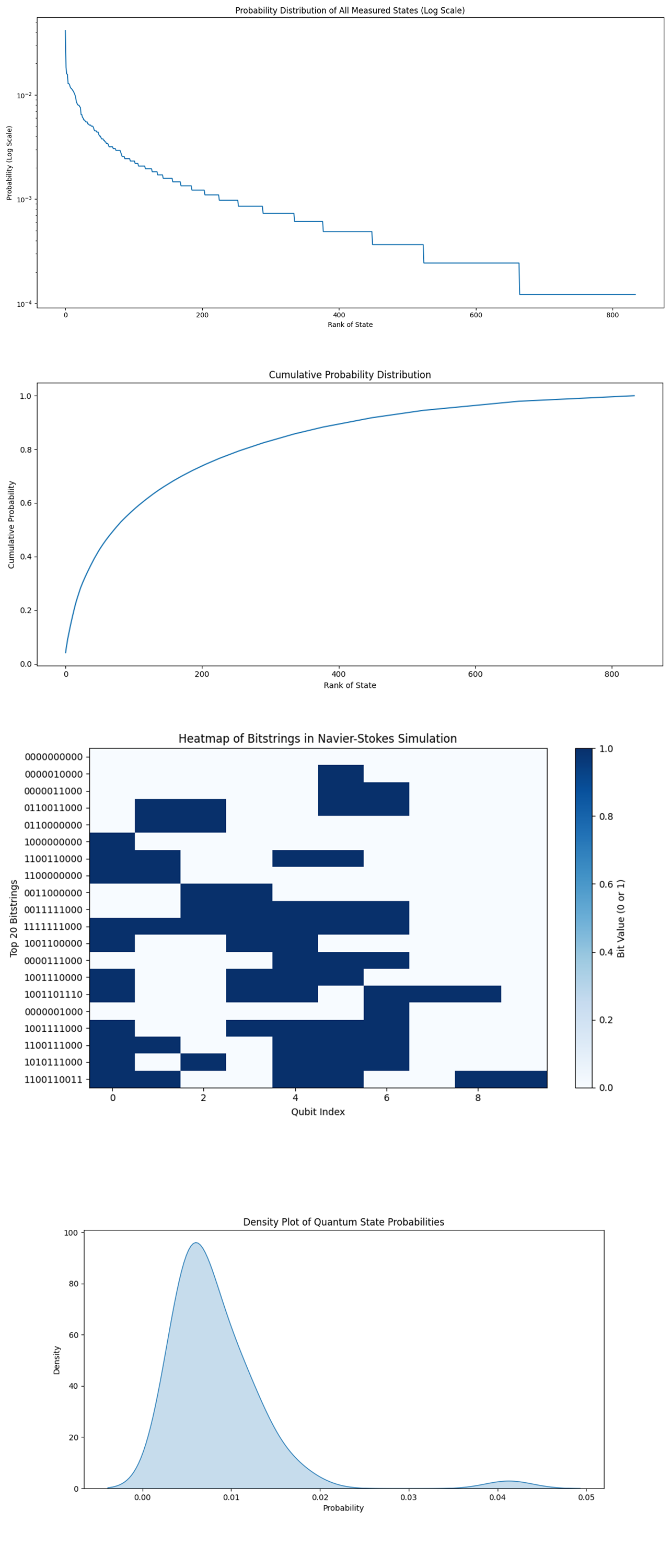
The Probability Distribution of All Measured States above (code below) provides a broader overview of the probability distribution of all the measured quantum states. The logarithmic scale shows how quickly the probabilities decrease as the states become less frequent. The curve demonstrates a rapid drop off, with only a few states having significant probabilities, while the majority of the states have much lower probabilities.
The rapid drop off in the probability distribution suggests that only a small number of fluid configurations are likely, with most states being rare or unstable. The presence of a long tail in the probability distribution reflects that there are many possible states, but they contribute very little to the overall dynamics of the system. This indicates that the quantum system, when simulating the fluid dynamics, favors certain states strongly over others, which may reflect the most stable or likely fluid flow patterns.
The Cumulative Probability Distribution above (code below) shows how quickly the probability mass is captured by the top states. The plot reveals that the top 200 states capture over 80% of the total probability mass, with the remaining states contributing marginally.
The fact that a small subset of states accounts for most of the total probability mass indicates that the fluid dynamics system is highly constrained to a few likely configurations. This could reflect the system's tendency to converge toward stable flow patterns under the linearized Navier-Stokes approximation.
The states beyond the top 200 contribute minimally to the overall dynamics, suggesting they represent rare or extreme fluid configurations that do not significantly affect the simulation's outcome.
The Heatmap above (code below) visualizes the top 20 quantum states as binary strings, with each row representing a bitstring (state) and each column corresponding to a qubit (or part of the fluid system). The color intensity shows whether a qubit is in the ∣0⟩ or ∣1⟩ state.
The first qubit (column 0) is predominantly in the ∣0⟩ state across the top states, indicating that it contributes heavily to stable fluid configurations. In contrast, qubits 1 and 2 exhibit more variability, reflecting local fluctuations in the fluid system. The heatmap highlights certain repeating patterns, such as clusters of qubits that frequently appear in the ∣1⟩ state together. These patterns suggest specific correlations between parts of the fluid system that evolve similarly.
The Density Plot of Quantum State Probabilities above (code below) shows a smoothed view of how the probabilities are distributed across all measured quantum states. The plot shows a sharp peak around low probability values, indicating that most of the quantum states have very small probabilities. The bulk of the probability mass is concentrated at low probabilities, with a long tail toward higher probabilities.
This plot confirms that only a small number of states carry most of the system's probability, while the majority of states are less likely to appear. This is reflective of the Navier-Stokes fluid system where the fluid dynamics are typically dominated by a few stable or low-energy configurations.

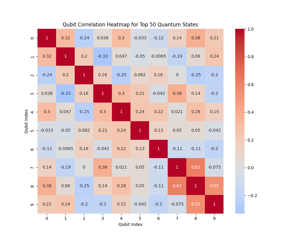
The Qubit Correlation Heatmap above (code below) shows the correlation between different qubits based on the top 50 quantum states, revealing how the states of the qubits are related to each other.
Several qubit pairs show strong positive correlations (highlighted by red blocks), meaning that these qubits tend to be in similar states (either both in ∣0⟩ or ∣1⟩) across the top quantum states. This suggests that these parts of the fluid system interact closely, reflecting localized fluid dynamics that are strongly coupled. Some qubit pairs exhibit negative correlations (blue blocks), indicating that when one qubit is in state ∣0⟩, the other is more likely to be in ∣1⟩. These negative correlations may reflect areas of the fluid system where counteracting forces or flows exist, akin to turbulent regions where fluid particles move in opposite directions.
The mixture of positive and negative correlations suggests a complex interaction between parts of the fluid system. While there are regions of stable, correlated flow (positive correlations), there are also areas of competing dynamics (negative correlations), which could correspond to fluid turbulence or complex interactions in the simulated flow.
In the end, through Carleman linearization, we were able to simulate a linear approximation of the Navier-Stokes equations. While this is not a direct solution to the full nonlinear Navier-Stokes equations, it provides an approximation of the system's behavior by embedding the nonlinear dynamics into a higher-dimensional linear system. Thus, we obtained an approximate solution to the fluid dynamics, focusing on the stable and most likely configurations. This quantum approach demonstrates the potential for quantum algorithms to tackle parts of such nonlinear problems.

Code:


# Imports
import numpy as np
import json
import matplotlib.pyplot as plt
from qiskit import QuantumCircuit, transpile
from qiskit_ibm_runtime import QiskitRuntimeService, Session, SamplerV2
import csv
import logging
from collections import Counter
from qiskit.visualization import plot_histogram

# Function to parse ECR error and extract the maximum error from multiple qubit pairs
def parse_ecr_error(ecr_error_str):
    qubit_error_pairs = ecr_error_str.split(';')
    errors = []
    for pair in qubit_error_pairs:
        qubit_pair, error_value = pair.split(':')
        errors.append(float(error_value))  # Convert the error value to a float
    return max(errors)  # Return the maximum error for simplicity

# Function to parse gate time and extract the maximum gate time from multiple qubit pairs
def parse_gate_time(gate_time_str):
    qubit_time_pairs = gate_time_str.split(';')
    times = []
    for pair in qubit_time_pairs:
        qubit_pair, time_value = pair.split(':')
        times.append(float(time_value))  # Convert the gate time value to a float
    return max(times)  # Return the maximum gate time 

# Load calibration data from CSV
def load_calibration_data(file_path):
    calibration_data = {}
    with open(file_path, mode='r') as file:
        reader = csv.DictReader(file)
        for row in reader:
            qubit = int(row['Qubit'])
            calibration_data[qubit] = {
                'T1': float(row['T1 (us)']) if row['T1 (us)'] else 0.0,
                'T2': float(row['T2 (us)']) if row['T2 (us)'] else 0.0,
                'readout_error': float(row['Readout assignment error ']) if row['Readout assignment error '] else 0.0,
                'sx_error': float(row['√x (sx) error ']) if row['√x (sx) error '] else 0.0,
                'pauli_x_error': float(row['Pauli-X error ']) if row['Pauli-X error '] else 0.0,
                'ecr_error': parse_ecr_error(row['ECR error ']) if row['ECR error '] else 0.0,  # Parse multiple ECR errors
                'gate_time': parse_gate_time(row['Gate time (ns)']) if row['Gate time (ns)'] else 0.0  # Parse multiple gate times
            }
    return calibration_data

# Select qubits with the best T1, T2, and error characteristics
def select_best_qubits(calibration_data, n_qubits):
    qubits_sorted = sorted(calibration_data.items(), key=lambda x: (x[1]['sx_error'], -x[1]['T1'], -x[1]['T2']))
    best_qubits = [qubit[0] for qubit in qubits_sorted[:n_qubits]]
    return best_qubits

# Create the quantum circuit for Navier-Stokes 
def create_navier_stokes_qc(n_qubits, time_step, orders):
    qc = QuantumCircuit(n_qubits, n_qubits)
    
    # Initial state preparation (using Ry rotations)
    for qubit in range(n_qubits):
        qc.ry(np.pi/4, qubit)
    
    # Carleman linearization gates (evolution)
    for step in range(orders):
        for qubit in range(n_qubits):
            qc.rz(np.pi / time_step, qubit)
        for qubit in range(n_qubits - 1):
            qc. cx(qubit, qubit + 1)
    
    # Measurement
    qc.measure(range(n_qubits), range(n_qubits))
    
    return qc

# IBMQ 
service = QiskitRuntimeService(
    channel='ibm_quantum',
    instance='ibm-q/open/main',
    token='YOUR_IBMQ_KEY_O-`'
)

backend_name = 'ibm_brisbane'
backend = service.backend(backend_name)

# Logging 
logging.basicConfig(level=logging. INFO)
logger = logging.getLogger(__name__)

# Load calibration data
calibration_file = '/Users/Documents/ibm_brisbane_calibrations_2024-10-22T20_46_34Z.csv'
calibration_data = load_calibration_data(calibration_file)

# Define the experiment parameters
n_qubits = 10
time_step = 0.1
orders = 3
shots = 8192

best_qubits = select_best_qubits(calibration_data, n_qubits)

# Transpile
qc = create_navier_stokes_qc(n_qubits, time_step, orders)
transpiled_qc = transpile(qc, backend=backend, optimization_level=3)

# Execute 
with Session(service=service, backend=backend) as session:
    sampler = SamplerV2(session=session)
    
    logger. info("Running the Navier-Stokes simulation on ibm_brisbane backend")
    job = sampler. run([transpiled_qc], shots=shots)
    job_result = job.result()

    # Measurement data 
    bit_array = job_result._pub_results[0]['__value__']['data'].c
    
    # Extract bitstrings
    bitstrings = bit_array.get_bitstrings()  # Extract the bitstrings using the correct method
    counts = dict(Counter(bitstrings))  # Count occurrences of each bitstring
    
    # Save the JSON
    results_data = {"raw_counts": counts}
    file_path = '/Users/Documents/NavierStokes_0.jso'
    with open(file_path, 'w') as f:
        json.dump(results_data, f, indent=4)

# Plot the results for analysis
plot_histogram(counts)
plt. show()

logger. info("Experiment complete.")

# End.

/////////////////////////////////////////////////////

Top 20 most Frequent States, Probability Distribution, Cumulative Probability Distribution, Heatmap of Bitstring Probabilities from Run Data
# Imports
import json
import numpy as np
import matplotlib.pyplot as plt
from collections import Counter

# Load the JSON
file_path = '/Users/Documents/NavierStokes_0.json'
with open(file_path, 'r') as file:
    data = json.load(file)

counts = data['raw_counts']
total_shots = sum(counts.values())

# Normalize counts to get probabilities
probabilities = {state: count / total_shots for state, count in counts.items()}

# Sort by probability to identify dominant states
sorted_probabilities = sorted(probabilities.items(), key=lambda x: x[1], reverse=True)

# Plotting the top 20 most frequent states
top_states = sorted_probabilities[:20]
states, probs = zip(*top_states)

plt.figure(figsize=(12, 6))
plt. bar(states, probs)
plt.xticks(rotation=90)
plt.xlabel('Bitstrings (Quantum States)')
plt.ylabel('Probability')
plt.title('Top 20 Quantum States in Navier-Stokes Simulation')
plt.tight_layout()
plt. show()

# Calculate Shannon Entropy
entropy = -sum(p * np.log2(p) for p in probabilities.values() if p > 0)  # Avoid log(0)
print(f"Shannon Entropy of the distribution: {entropy:.4f}")

# Plot full probability distribution (log scale)
plt.figure(figsize=(14, 7))
all_states, all_probs = zip(*sorted_probabilities)
plt.plot(range(len(all_probs)), all_probs)
plt.yscale('log')
plt.xlabel('Rank of State')
plt.ylabel('Probability (Log Scale)')
plt.title('Probability Distribution of All Measured States (Log Scale)')
plt.tight_layout()
plt. show()

# Cumulative Probability Distribution
cumulative_probs = np.cumsum(all_probs)
plt.figure(figsize=(12, 6))
plt.plot(range(len(cumulative_probs)), cumulative_probs)
plt.xlabel('Rank of State')
plt.ylabel('Cumulative Probability')
plt.title('Cumulative Probability Distribution')
plt.tight_layout()
plt. show()

#  Heatmap of Bitstring Probabilities
bitstrings_matrix = np.array([list(map(int, state)) for state in all_states[:20]])  # Convert top 20 bitstrings to binary matrix
plt.figure(figsize=(10, 6))
plt.imshow(bitstrings_matrix, cmap='Blues', aspect='auto')
plt.colorbar(label='Bit Value (0 or 1)')
plt.yticks(range(len(states)), states)
plt.xlabel('Qubit Index')
plt.ylabel('Top 20 Bitstrings')
plt.title('Heatmap of Bitstrings in Navier-Stokes Simulation')
plt.tight_layout()
plt. show()

//////////////////////////////////////////////////
Density Plot of Probabilities, Correlation Heatmap (Bitwise Analysis) from Run Data
# Imports
import json
import numpy as np
import matplotlib.pyplot as plt
from collections import Counter
from mpl_toolkits.mplot3d import Axes3D
import seaborn as sns

# Load the results from the JSON file
file_path = '/Users/Documents/NavierStokes_0.json'
with open(file_path, 'r') as file:
    data = json.load(file)

counts = data['raw_counts']
total_shots = sum(counts.values())

# Normalize counts to get probabilities
probabilities = {state: count / total_shots for state, count in counts.items()}

# Sort by probability to identify dominant states
sorted_probabilities = sorted(probabilities.items(), key=lambda x: x[1], reverse=True)

# Prepare data for 3D visualization
top_n = 50
states, probs = zip(*sorted_probabilities[:top_n])

# Convert bitstrings to integers 
int_states = [int(state, 2) for state in states]

# Density Plot of Probabilities
plt.figure(figsize=(12, 6))
sns.kdeplot(probs, shade=True)
plt.title('Density Plot of Quantum State Probabilities')
plt.xlabel('Probability')
plt.ylabel('Density')
plt. show()

# Correlation Heatmap (Bitwise Analysis)
# Convert top 50 bitstrings into a binary matrix
bitstrings_matrix = np.array([list(map(int, state)) for state in states])

# Compute correlation between each qubit pair
corr_matrix = np.corrcoef(bitstrings_matrix.T)

plt.figure(figsize=(10, 8))
sns.heatmap(corr_matrix, annot=True, cmap='coolwarm', center=0)
plt.title('Qubit Correlation Heatmap for Top 50 Quantum States')
plt.xlabel('Qubit Index')
plt.ylabel('Qubit Index')
plt. show()

# End