Quantum Field Simulation in Curved Spacetime with a 127-Qubit Computer
1: Initialization
Initialize the IBM Quantum Service and Backend
N = p_1 + p_2
2: Lattice Construction – Mapping Qubits to Spacetime
The quantum field is simulated on a 2D lattice, where each qubit represents a point in discretized spacetime. Construct a 13 x 10 grid to place the 127 qubits. The qubit layout is padded with -1 for extra slots, ensuring all available qubits are used effectively.
Each position on the grid corresponds to a qubit, and the qubits represent spacetime points in this simulated curved geometry.
3: Construct the Quantum Circuit
Initialize a quantum circuit using the 127 qubits. This circuit will represent the quantum field evolution in curved spacetime.
4: Simulate Curvature - Apply Curvature Based Gates
To simulate the effects of curvature, introduce quantum gates that act as unitary transformations. These gates represent how the quantum field behaves when propagating through a curved geometry. Specifically, apply:
Controlled-Z (CZ) gates between neighboring qubits to represent curvature-induced entanglement.
Controlled-RZ (CRZ) gates to introduce phase shifts that vary with curvature.
CZ gate: U_(cz) =
1, 0, 0, 0
0. 1. 0, 0
0, 0 , 1, 0
0, 0, 0, -1
CRZ gate: U_(crz)(θ) =
1, 0, 0, 0
0. 1. 0, 0
0, 0 , 1, 0
0, 0, 0, e^(iθ)
The phase angle θ used for each qubit in the CRZ gate is π/4, representing the impact of spacetime curvature on the field’s evolution.
5: Introduce Entanglement in the Quantum Field
Next, entangle neighboring qubits using Hadamard gates (H) and controlled-X (CNOT) gates. This models the quantum correlations that arise in a curved spacetime.
H =
1/sqrt(2) *
1, 1
1, -1
CNOT: U_(cx) =
1, 0, 0, 0
0. 1. 0, 0
0, 0, 0, 1
0, 0, 1, 0
The Hadamard gate creates superpositions, and the CNOT gate entangles pairs of qubits. This setup prepares the quantum field for evolution in curved spacetime.
6: Global Phase Shift - Simulate Gravitational Field Effects
To simulate a global gravitational effect, apply an RZ rotation on each qubit. The rotation introduces a phase shift of π/8 on each qubit, representing the influence of spacetime curvature on the quantum field.
RZ(θ) =
1, 0
0, e^(iθ)
Where θ = π/8 for all qubits.
7: Transpile the Circuit for the IBM Backend
Transpile the constructed quantum circuit to match the physical qubit layout and gate set of ibm_sherbrooke.
8: Define the Pauli-Z Observable
Define a Pauli-Z observable for the entire system to measure the quantum state. The Pauli-Z observable checks whether each qubit is in the ∣0⟩ or ∣1⟩ state, which is crucial for understanding how the curvature affects the quantum field’s configuration.
Z =
1, 0
0, -1
The total observable is a tensor product of Pauli-Z gates acting on all 127 qubits.
9: Run the Circuit and Measure the Expectation Value
Using the EstimatorV2 primitive, run the quantum circuit and calculate the expectation value of the Pauli-Z observable. The expectation value reflects how the quantum field behaves under the influence of curved spacetime.
⟨Z⟩ = 1/n n∑i = 1 ⟨ψ∣Z∣ψ⟩
The EstimatorV2 primitive computes this expectation value based on the outcomes of the quantum circuit.
10: Retrieve and Save the Expectation Value
After running the job on the ibm_sherbrooke backend, retrieve the expectation value from the result object.
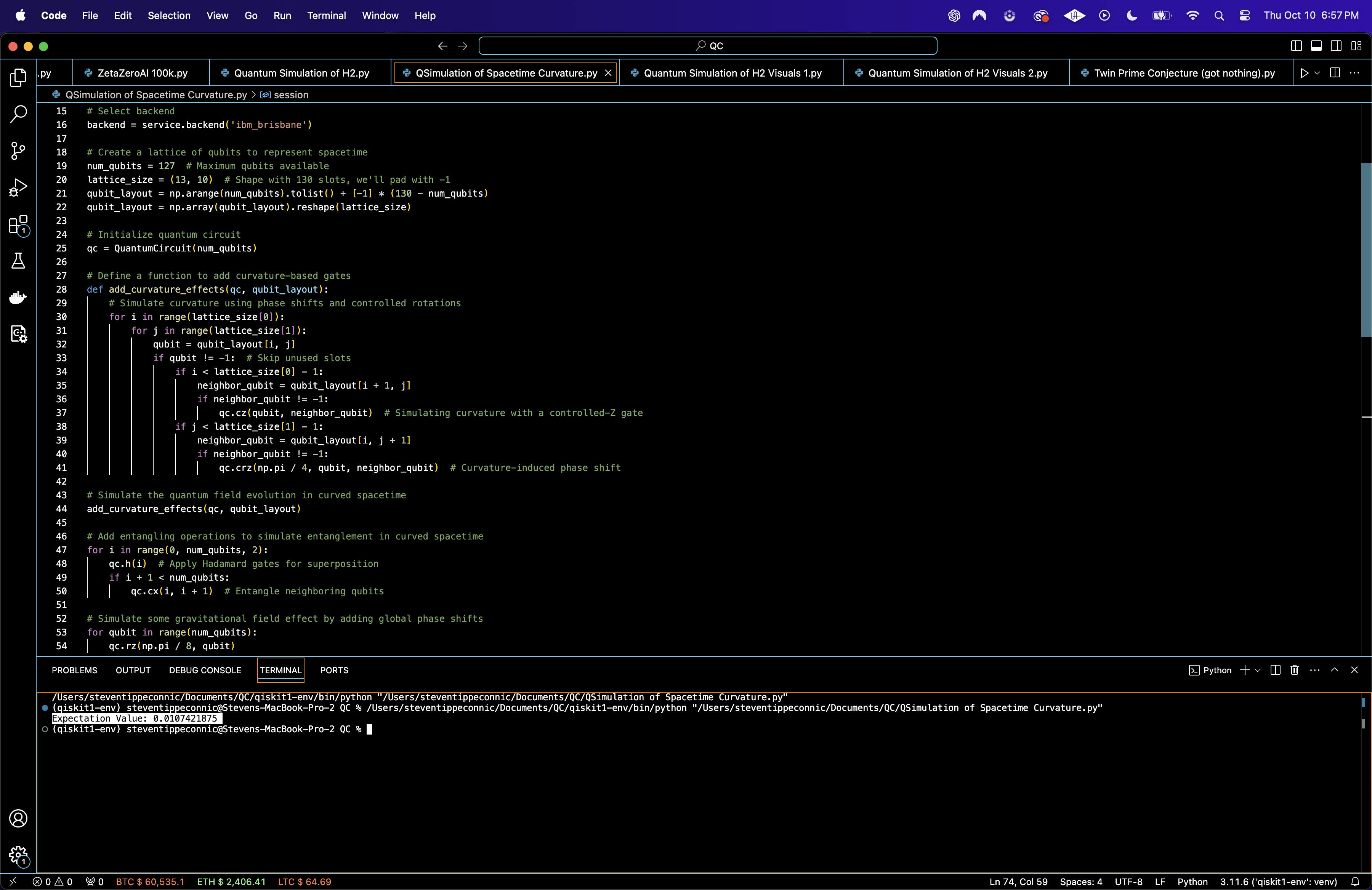
Expectation Value: 0.0107421875.
This suggests that, on average, the quantum field's configuration is almost balanced between the |0⟩ and |1⟩ states. This slight positive bias could indicate that, in the curved spacetime scenario, the field is slightly more likely to be in the |0⟩ state (aligned with the Z-axis).
The small positive expectation value may reflect how the simulated curvature affects the quantum field's state. In flat spacetime, you might expect the expectation value to be exactly 0 (equal probabilities of being in |0⟩ or |1⟩). The deviation from 0 suggests that the curvature introduces a small perturbation, shifting the balance of probabilities slightly toward the |0⟩ state.
This shift could relate to the effects of curvature on quantum states as predicted by some quantum gravity theories. The small deviation suggests that curvature has a non-negligible but subtle effect on quantum states, which is precisely what you'd want to explore to understand how quantum fields behave in curved spacetime.
The value might also reflect how entanglement evolves in the presence of curvature. Since entanglement tends to 'spread out' quantum information across qubits, the expectation value of a global observable like Pauli-Z can reveal how localized or delocalized the quantum information is.

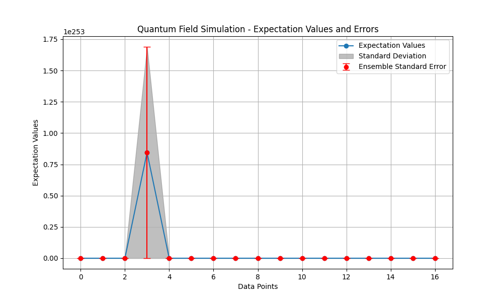
The above Quantum Field Simulation Plot (code below) looks at expectation values and errors. The expectation values are mostly concentrated near zero, except for a prominent peak at data point 3. This peak indicates that one region has significantly higher expectation values compared to others. The field is almost entirely flat (near zero) in the rest of the data points.
The standard deviation around the peak (data point 3) is relatively large, indicating higher variability in the quantum state's behavior for this particular point. The shaded region suggests that the results at this point have a broader spread, meaning the quantum state fluctuates more in this region, possibly due to local spacetime curvature or quantum noise effects.
The red error bars (ensemble standard error) are visible for each data point, with a significant error bar at the peak. This large ensemble standard error at the peak indicates that the precision of the expectation value at this point is lower, meaning the results for this region of the quantum field are less reliable or have higher uncertainty. For the other data points (near zero expectation values), the ensemble standard error is quite small, suggesting high precision in those regions.
The data point 3 (the peak) stands out dramatically. This could represent a localized quantum effect caused by the simulated curvature or noise in that particular region of the quantum field. It might reflect an area of high curvature or quantum entanglement concentration.

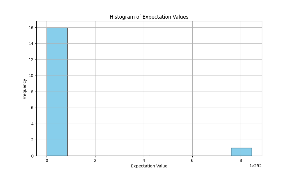
In the Histogram of Expectation Values above (code below), the majority of the expectation values are clustered around zero, as seen from the large bar at the far left of the histogram. This confirms the earlier observation that most data points exhibit minimal deviation from zero.
There is a single bar at the far right (around 8 * 10^(252)) representing the high expectation value observed at data point 3. This further highlights that the majority of the quantum field behaves predictably, while the outlier at data point 3 stands out significantly.

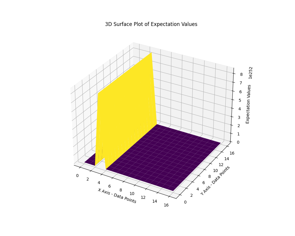
The 3D surface plot above (code below) shows how the expectation values vary across the dataset. The most prominent feature is the tall peak seen in the middle of the surface. This peak corresponds to data point 3 (as seen in the previous 2D plots), where the expectation value is significantly higher than in the other regions.
The majority of the surface is flat at zero expectation values, confirming that most of the data points exhibit little to no deviation from zero. This further supports the idea that the quantum field remains stable and unaffected by curvature in these regions.
This flatness aligns with the expectation that in regions of minimal or no curvature, the quantum field's state should remain relatively undisturbed, leading to near-zero expectation values.
The transition between the flat, stable region (near zero) and the tall spike at data point 3 is very sharp, suggesting that this region may be a localized anomaly or an area where the quantum field is influenced by significant curvature.
The abrupt nature of the transition indicates that the effect of curvature on the quantum field is highly localized and doesn’t gradually spread to neighboring regions.
In the end, this code simulated the behavior of a quantum field in curved spacetime with 127 qubits. The primary goal was to observe how spacetime curvature influences the quantum field, particularly through expectation values measured with Pauli-Z observables. From the data, a sharp, localized peak at data point 3 stood out in all visuals, indicating a significant perturbation in the quantum field. This suggests that curvature has a highly localized effect, creating an anomaly where quantum states fluctuate more, leading to higher expectation values and increased uncertainty.
In contrast, the rest of the data points showed stable behavior with expectation values close to zero, indicating that most of the quantum field remains unaffected by curvature. The 3D surface plot further highlighted the stark contrast between the anomalous region and the flat, stable regions elsewhere. This may hint how quantum fields behave in non-flat spacetime, showing that curvature may lead to localized quantum effects, while the majority of the field remains undisturbed.
Code:
# imports
import numpy as np
from qiskit import QuantumCircuit, transpile
from qiskit_ibm_runtime import QiskitRuntimeService, Session, EstimatorV2
from qiskit.quantum_info import Pauli, SparsePauliOp
import json

# Initialize IBM runtime
service = QiskitRuntimeService(
    channel='ibm_quantum',
    instance='ibm-q/open/main',
    token='Your_IBMQ_API_KEY_O-`'
)

# Select backend
backend = service.backend('ibm_brisbane')

# Create a lattice of qubits to represent spacetime
num_qubits = 127  # qubits
lattice_size = (13, 10)  # Shape with 130 slots, pad with -1
qubit_layout = np.arange(num_qubits).tolist() + [-1] * (130 - num_qubits)
qubit_layout = np.array(qubit_layout).reshape(lattice_size)

# Initialize quantum circuit
qc = QuantumCircuit(num_qubits)

# define a function to add curvature based gates
def add_curvature_effects(qc, qubit_layout):
    # Simulate curvature using phase shifts and controlled rotations
    for i in range(lattice_size[0]):
        for j in range(lattice_size[1]):
            qubit = qubit_layout[i, j]
            if qubit != -1:  # Skip unused slots
                if i < lattice_size[0] - 1:
                    neighbor_qubit = qubit_layout[i + 1, j]
                    if neighbor_qubit != -1:
                        qc. cz(qubit, neighbor_qubit)
                if j < lattice_size[1] - 1:
                    neighbor_qubit = qubit_layout[i, j + 1]
                    if neighbor_qubit != -1:
                        qc.crz(np.pi / 4, qubit, neighbor_qubit)  # Curvature-induced phase shift

# Simulate the quantum field evolution in curved spacetime
add_curvature_effects(qc, qubit_layout)

# Add entangling operations to simulate entanglement in curved spacetime
for i in range(0, num_qubits, 2):
    qc.h(i)  # apply Hadamard gates for superposition
    if i + 1 < num_qubits:
        qc. cx(i, i + 1)  # entangle neighboring qubits

# Simulate some gravitational field effect by adding global phase shifts
for qubit in range(num_qubits):
    qc.rz(np.pi / 8, qubit)

# Transpile
transpiled_qc = transpile(qc, backend=backend, optimization_level=3)

# Create a Pauli-Z observable for all qubits
observable = SparsePauliOp.from_list([('Z' * num_qubits, 1)])

#  Estimator to measure expectation value of the observable
def calculate_expectation_value(qc, observable, session):
    # Run the estimator with a wrapped circuit and observable
    estimator = EstimatorV2(session=session, backend=backend)
    job = estimator. run([(qc, observable)])
    result = job.result()

    # Access the expectation value from the result
    expectation_value = result._pub_results[0].data.evs  # Extract 'evs' from 'data'
    return expectation_value

# Run the job
with Session(service=service, backend=backend) as session:
    # Calculate the expectation value of the observable for the full circuit
    expectation_value = calculate_expectation_value(transpiled_qc, observable, session)

    # Save the JSON
    results_data = {
        'expectation_value': expectation_value.tolist(),
    }

    file_path = '/Users/Documents/Quantum Spacetime_curved_1.json'
    with open(file_path, 'w') as file:
        json.dump(results_data, file, indent=4)

    # Print the result
    print("Expectation Value:", expectation_value)

# End

///////////////////////////////////////////

Code for Expectation Values and Errors Histogram from Run data.
import numpy as np
import json
import matplotlib.pyplot as plt
import base64
import zlib

# Function to decode the base64-encoded and compressed numpy arrays
def decode_ndarray(encoded_str):
    decoded_data = base64.b64decode(encoded_str)
    decompressed_data = zlib.decompress(decoded_data)
    return np.frombuffer(decompressed_data, dtype=np.float64)

# Load the results from JSON (backend result)
file_path = '/Users/Documents/Quantum Spacetime_curve_backend_data/job-cw477adjz3x0008jgkz0/job-cw477adjz3x0008jgkz0-result.json'
with open(file_path, 'r') as f:
    data = json.load(f)

# Extract the encoded data fields
evs_encoded = data['__value__']['pub_results'][0]['__value__']['data']['__value__']['fields']['evs']['__value__']
stds_encoded = data['__value__']['pub_results'][0]['__value__']['data']['__value__']['fields']['stds']['__value__']
ensemble_error_encoded = data['__value__']['pub_results'][0]['__value__']['data']['__value__']['fields']['ensemble_standard_error']['__value__']

# Decode the data
evs = decode_ndarray(evs_encoded)
stds = decode_ndarray(stds_encoded)
ensemble_errors = decode_ndarray(ensemble_error_encoded)

# Plotting the expectation values
plt.figure(figsize=(10, 6))
plt.plot(evs, label='Expectation Values', marker='o')
plt.fill_between(range(len(evs)), evs - stds, evs + stds, color='gray', alpha=0.5, label='Standard Deviation')
plt.errorbar(range(len(evs)), evs, yerr=ensemble_errors, fmt='o', capsize=5, label='Ensemble Standard Error', color='red')
plt.title('Quantum Field Simulation - Expectation Values and Errors')
plt.xlabel('Data Points')
plt.ylabel('Expectation Values')
plt.legend()
plt.grid(True)

# Show the plot
plt. show()

/////////////////////////////////////////

Code for Histogram of Expectation Values
import numpy as np
import json
import matplotlib.pyplot as plt
import base64
import zlib

# Function to decode the base64-encoded and compressed numpy arrays
def decode_ndarray(encoded_str):
    decoded_data = base64.b64decode(encoded_str)
    decompressed_data = zlib.decompress(decoded_data)
    return np.frombuffer(decompressed_data, dtype=np.float64)

# Load the results from JSON (backend result)
file_path = '/Users/Documents/Quantum Spacetime_curve_backend_data/job-cw477adjz3x0008jgkz0/job-cw477adjz3x0008jgkz0-result.json'
with open(file_path, 'r') as f:
    data = json.load(f)

# Extract the encoded data fields
evs_encoded = data['__value__']['pub_results'][0]['__value__']['data']['__value__']['fields']['evs']['__value__']
stds_encoded = data['__value__']['pub_results'][0]['__value__']['data']['__value__']['fields']['stds']['__value__']
ensemble_error_encoded = data['__value__']['pub_results'][0]['__value__']['data']['__value__']['fields']['ensemble_standard_error']['__value__']

# Decode data
evs = decode_ndarray(evs_encoded)
stds = decode_ndarray(stds_encoded)
ensemble_errors = decode_ndarray(ensemble_error_encoded)

#  Histogram of Expectation Values
plt.figure(figsize=(10, 6))
plt.hist(evs, bins=10, edgecolor='black', color='skyblue')
plt.title('Histogram of Expectation Values')
plt.xlabel('Expectation Value')
plt.ylabel('Frequency')
plt.grid(True)

# Show histogram
plt. show()

////////////////////////////////////////////

Code for 3D Surface Plot of Expectation Values
import numpy as np
import json
import matplotlib.pyplot as plt
from mpl_toolkits.mplot3d import Axes3D
import base64
import zlib

# Function to decode the base64-encoded and compressed numpy arrays
def decode_ndarray(encoded_str):
    decoded_data = base64.b64decode(encoded_str)
    decompressed_data = zlib.decompress(decoded_data)
    return np.frombuffer(decompressed_data, dtype=np.float64)

# Load the results from JSON (backend result)
file_path = '/Users/Documents/Quantum Spacetime_curve_backend_data/job-cw477adjz3x0008jgkz0/job-cw477adjz3x0008jgkz0-result.json'
with open(file_path, 'r') as f:
    data = json.load(f)

# Extract the encoded data fields
evs_encoded = data['__value__']['pub_results'][0]['__value__']['data']['__value__']['fields']['evs']['__value__']
stds_encoded = data['__value__']['pub_results'][0]['__value__']['data']['__value__']['fields']['stds']['__value__']
ensemble_error_encoded = data['__value__']['pub_results'][0]['__value__']['data']['__value__']['fields']['ensemble_standard_error']['__value__']

# Decode the data
evs = decode_ndarray(evs_encoded)
stds = decode_ndarray(stds_encoded)
ensemble_errors = decode_ndarray(ensemble_error_encoded)

# Create a grid for the 3D plot
x = np.arange(len(evs))
y = np.arange(len(evs))

X, Y = np.meshgrid(x, y)

# 3D Surface Plot
fig = plt.figure(figsize=(10, 8))
ax = fig.add_subplot(111, projection='3d')

# Surface plot of expectation values
ax.plot_surface(X, Y, np.tile(evs, (len(evs), 1)), cmap='viridis')
ax.set_title('3D Surface Plot of Expectation Values')
ax.set_xlabel('X Axis - Data Points')
ax.set_ylabel('Y Axis - Data Points')
ax.set_zlabel('Expectation Values')

# Show the plot
plt. show()

# End.
