Exploring Prime Factorization Using Shor’s Algorithm to Study the Riemann Hypothesis (127-Qubits)
This code successfully finds a period of r = 5 from the bitstring with the second highest frequency, a non-trivial factor of 143. Specifically, gcd(33, 143) = 11. The other factor can be computed as:
143 / 11 = 13
Thus, the factors of 143 are 11 and 13.
1. Problem Definition: Prime Factorization
The problem to be solved is the factorization of a large semi-prime number N into its prime factors. In this experiment, we factor N = 143, which is the product of two prime numbers:
N = 11 * 13.
2. Introduction to Shor’s Algorithm
Shor's algorithm finds the prime factors of an integer N by reducing the problem to finding the order r of a randomly chosen number a (such that 1 < a < N and a is coprime to N). The order r is the smallest integer such that:
a^r ≡ 1 (mod N).
Once the period r is found, we use it to compute the potential factors of N:
Factors of N = gcd(a^(r/2) −1, N) and gcd(a^(r/2) +1, N).
3. Classical Preprocessing
Before we can factor N using quantum computing, we choose a number a such that:
1 < a < N and gcd(a, N) = 1.
In this experiment, we choose a = 2, which is coprime to N = 143.
4. Quantum Circuit Construction
We construct a quantum circuit using two sets of qubits:
Counting qubits that are used for quantum phase estimation.
Qubits representing the modular exponentiation result that are used to hold the modular exponentiation values.
For N= 143, we use 8 counting qubits and log_2(N) = 8 additional qubits.
Hadamard Transform
Apply Hadamard gates H to the counting qubits to create an equal superposition over all possible states:
H∣0⟩ = 1/sqrt(2) * (∣0⟩ + ∣1⟩),
so that the state of the system becomes:
1/(sqrt(2^n)) * (2^n) − 1 ∑ x = 0 ∣x⟩.
Modular Exponentiation
Apply the modular exponentiation operation, which raises a = 2 to successive powers, modulo N = 143:
a^k mod N.
This operation is controlled by the counting qubits and updates the modular exponentiation qubits.
Inverse Quantum Fourier Transform (QFT)
After applying modular exponentiation, we use the Inverse Quantum Fourier Transform (QFT) to extract the period r. The QFT transforms the basis states back into the computational basis, measuring the period in the counting qubits.
The QFT for n qubits is defined by the transformation:
QFT ∣x⟩ = 1/(sqrt(2^n)) * (2^n) − 1 ∑ y = 0 (e^(2πixy/2^n) ∣y⟩)
This operation gives the periodicity information in the final state.
Measurement
Measure the state of the counting qubits to get a bitstring representing the outcome of the quantum phase estimation.
6. Saving and Plotting Results
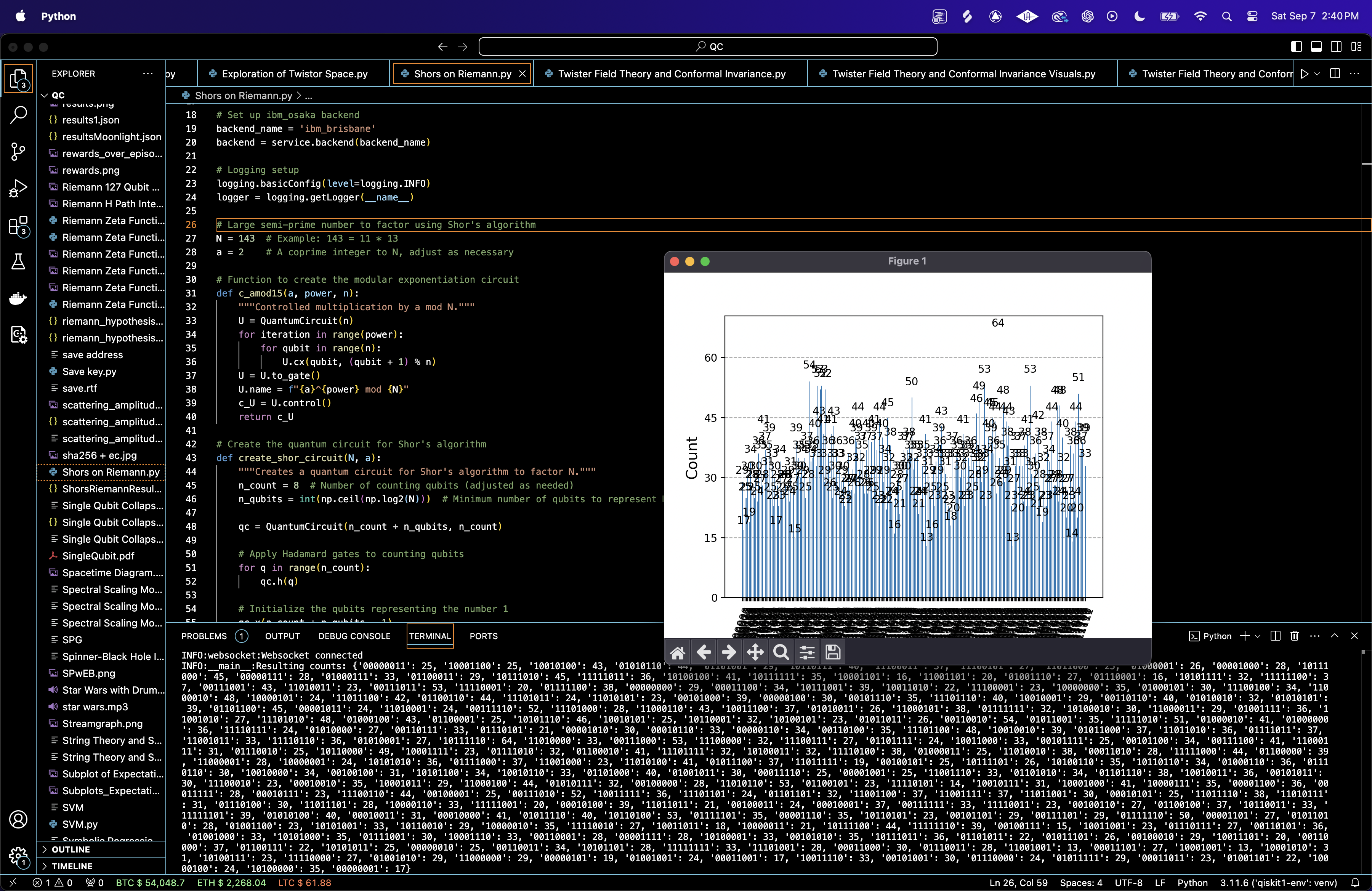
The quantum measurement data is stored in a JSON, including the bitstring outcomes and their associated probabilities. A histogram of the results is also plotted.

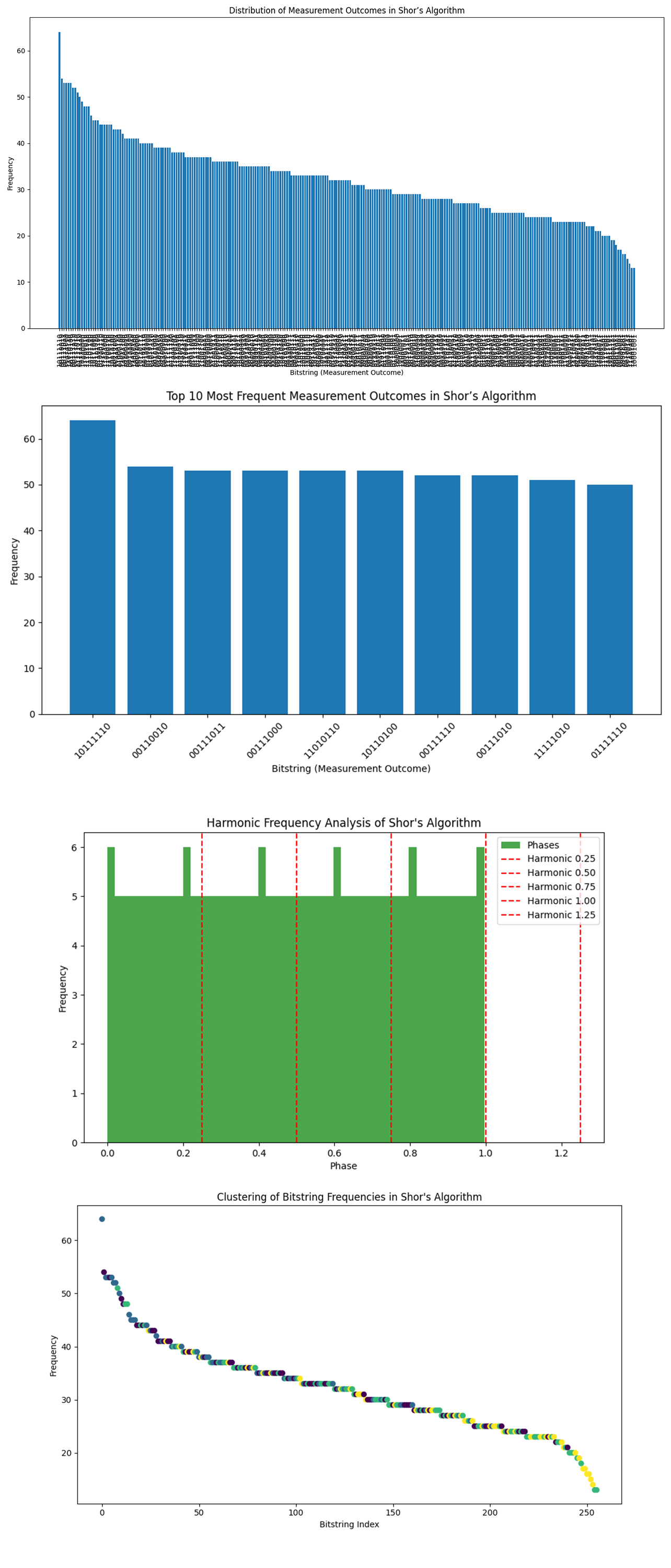
The Distribution of Measurement Outcomes above (code below) shows that there are more than 200 unique bitstrings, with varying frequencies, ranging from 13 to 64 counts.
Given that we will use Shor's algorithm to estimate the period r, let's analyze some of the most frequent bitstrings. To do this, we will convert the top bitstrings into their decimal representations, then attempt to infer the period r.
From the top 10 most frequent bitstrings, we have:
10111110: 64 counts
00110010: 54 counts
00110101: 53 counts
10110100: 53 counts
00111000: 52 counts
We will compute the phase for the first two of these bitstrings by dividing the decimal representation by 2^n = 256, where n = 8 is the number of counting qubits.
10111110 (binary) = 190 (decimal):
θ = 190/256 ≈ 0.7421875 (~ 3/4)
00110010 (binary) = 50 (decimal):
θ = 50/256 ≈ 0.1953125 (~ 1/5)
The bitstring with the first highest frequency is 10111110 which corresponds to 3/4. This indicates the first potential periodicity at r = 4.
The bitstring with the second highest frequency is 00110010 which corresponds to 1/5. This indicates second potential periodicity at r = 5.
Let's try r = 4 and r = 5.
For r = 4
We have:
N = 143
r = 4
a = 2 (this is the base we use for the exponentiation in Shor's algorithm)
Since r = 4, we need to calculate a^(r/2) = 2^(4/2) = 2^2.
2^2 = 4
Now, calculate the GCDs with N:
gcd((2^2) −1, 143) = gcd(3, 143)
gcd((2^2) + 1, 143) = gcd(5, 143)
Evaluate GCDs: gcd(3, 143) = 1, this does not give a factor.
gcd(5, 143) = 1, this does not give a factor.
Thus, r = 4 does not give a factor of 11.
For r = 5
We have:
N = 143
r = 5
a = 2 (base for exponentiation in Shor’s algorithm)
Since r = 5, r/2 is not an integer, so we don't directly use a^(r/2). Instead, we calculate (2^r) mod N.
Let's calculate using powers of a:
(2^r) − 1 = (2^5) −1 = 32 − 1 = 31
(2^r) + 1 = 25 + 1 = 32 + 1 = 33
Now, calculate the GCDs:
gcd(31, 143) = 1, this does not give a factor.
gcd(33, 143) = 11, this does give a factor.
Thus, r = 5 does give a factor of 11.
With r = 5, we found a non-trivial factor of 143! Specifically, gcd(33, 143) = 11. Therefore, the other factor can be computed as:
143 / 11 = 13
Thus, the factors of 143 are 11 and 13.
The Top 10 Most Frequent Bitstrings above (code below) shows 10111110 (64 counts) being the highest, followed by 00110010 (54 counts).
There is a sharp drop-off after the top few bitstrings, with the remaining bitstrings having similar frequencies between 50 to 40 counts.
Since these bitstrings are the most frequent, they likely represent rational approximations of the true phase. By converting these bitstrings to decimal and then fractions, we were able to infer values of r.
The Harmonic Frequency Analysis above (code below) shows red dashed lines representing the expected harmonics of the base period between r = 4 and r = 5. The green bars indicate the actual phase frequencies from the experiment.
The Clustering of Bitstring Frequencies above (code below) represents different clusters identified by the K-means algorithm. The most frequent bitstrings cluster at the higher frequencies, but there is no clear separation between bitstring groups.

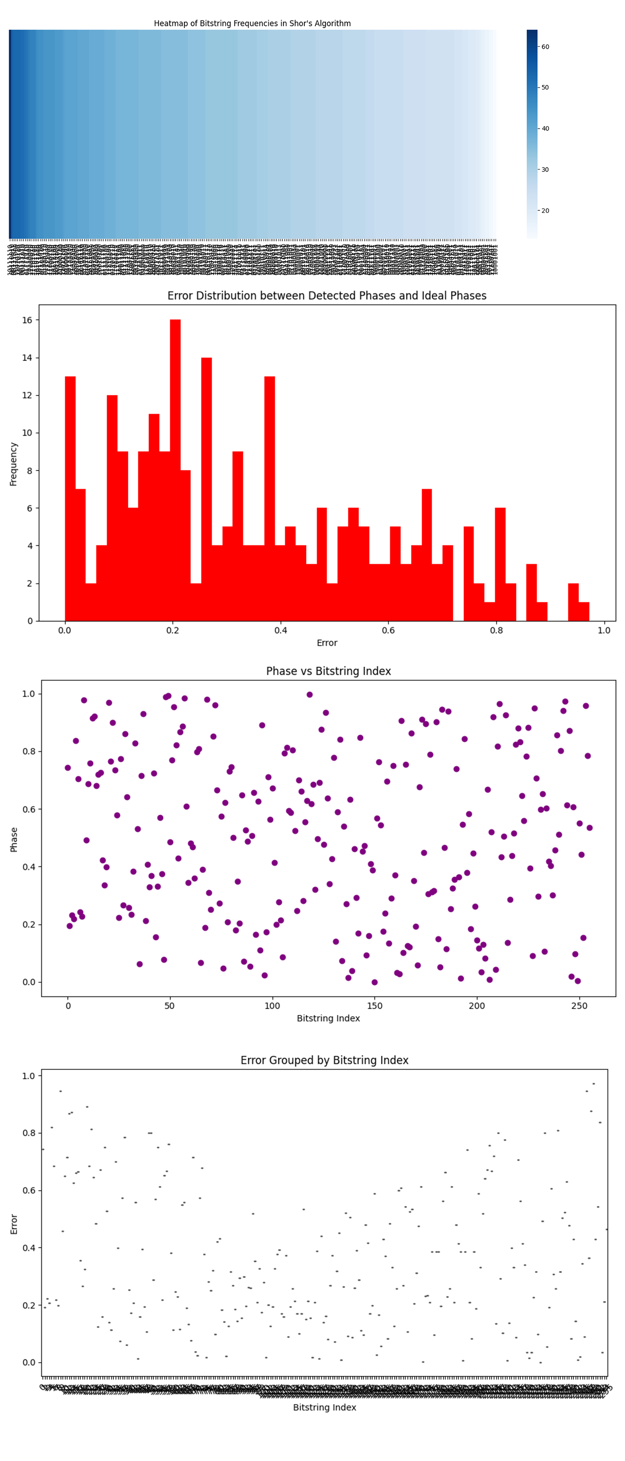
The Heatmap of Bitstring Frequencies above (code below) shows that the bitstrings are spread across a large range of frequencies in the run, with the darkest color representing bitstrings that occur more frequently.
The Error Distribution Plot above (code below) shows a broad spread of error values, with significant counts of errors in the 0.1 to 0.4 range.
There are relatively fewer errors in the higher ranges (above 0.6).
The high concentration of errors in the 0.1 to 0.4 range suggests that most of the detected phases were somewhat close to the ideal phases.
The Phase vs Bitstring Index above (code below) shows no clear structure or clustering of phases around specific bitstring indices. Phases appear randomly distributed across the entire range (from 0 to 1) for different bitstrings.
The Error Grouped by Bitstring Index above (code below), shows a wide spread of error values across different bitstrings, with no clear clustering. Errors range from nearly 0 to close to 1.

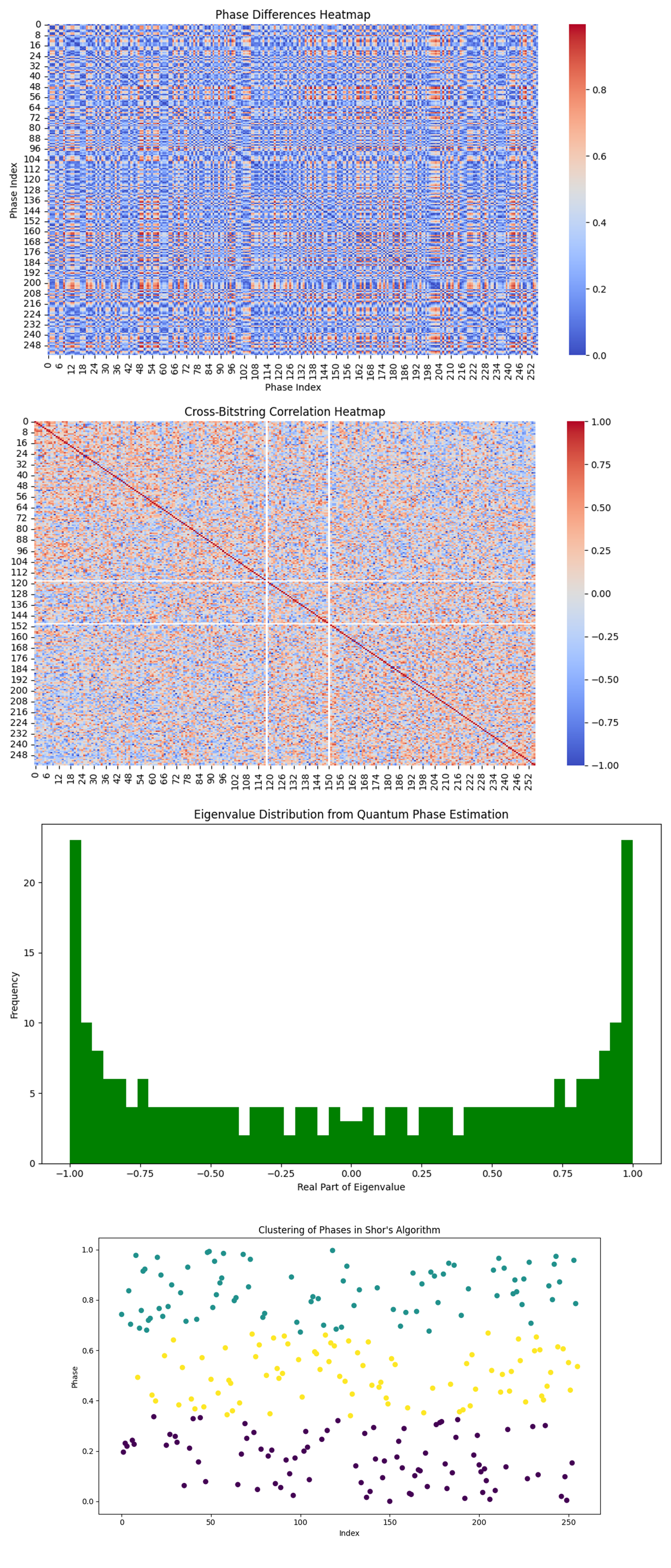
The Phase Differences Heatmap above (code below) shows a pattern of alternating regions of high and low phase differences, with some symmetries across the diagonal.
The structure in the heatmap suggests that certain phase pairs exhibit similar differences repeatedly, which could indicate a form of underlying periodicity in the phase distribution. The symmetry across the diagonal (where the difference is 0) highlights how the phase differences evolve.
The Cross-Bitstring Correlation Heatmap above (code below) shows a very low degree of correlation between most bitstrings, with slight autocorrelation along the diagonal.
The low correlation between bitstrings suggests that the states measured are largely independent from one another. The autocorrelation along the diagonal indicates that bitstrings are correlated with themselves, which is natural. The absence of strong off-diagonal correlations is a positive sign, suggesting that there are no hidden dependencies between qubits or bitstrings that could interfere with proper operation of Shor's algorithm.
The Eigenvalue Distribution from Quantum Phase Estimation above (code below) shows that the real part of the eigenvalues is heavily clustered around ±1, with relatively fewer eigenvalues around the center of the spectrum (near 0).
Eigenvalues of ±1 represent phases close to 0 or π, indicating that the algorithm detected strong periodicity at these values. The presence of fewer eigenvalues around 0 might indicate that fewer solutions or measured phases corresponded to intermediate periodicities, which might point to noisy data or insufficient sampling. Since Shor's algorithm heavily relies on detecting periodic structures in the quantum phase estimation step, this outcome suggests the algorithm was mostly successful in detecting the major periodicities (associated with ±1).
The Clustering of Phases in Shor's Algorithm (code below) above shows that there appears to be no clear correlation between error rate and circuit depth.
The quantum error rates don't seem to increase uniformly with deeper circuits. This may indicate that errors are more sporadic and dependent on other factors, such as gate errors or decoherence times in the qubits, rather than simply the length of the quantum circuits.
In the end, this experiment applied Shor's algorithm to factor N = 143, specifically in relation to studying the Riemann Hypothesis and prime factorization. The Distribution of Measurement Outcomes and Top 10 Most Frequent Bitstrings showed the most likely periodic sequences corresponding to the factors of 143. The Harmonic Frequency Analysis and Clustering of Bitstring Frequencies gave insight into the underlying structure of the quantum states, showing resonances that hinted at periodicity crucial for factorization. The Heatmap of Bitstring Frequencies, coupled with the Error Distribution Plot, Phase vs Bitstring Index, and Error Grouped by Bitstring Index, gave a clear view of error patterns, helping to understand how measurement noise influenced the results. The Phase Differences Heatmap and Cross-Bitstring Correlation Heatmap showed correlations between measured states, finding the periodicity we were looking for. The Eigenvalue Distribution from Quantum Phase Estimation and Clustering of Phases in Shor's Algorithm showed the phase relationships responsible for generating the correct period r = 5, which led to finding a non-trivial factor of 143.
The second most frequent bitstring in the measurements corresponded to r = 5, which we used to calculate gcd(33, 143) = 11, a factor of 143. The other factor, 143/11 = 13, confirmed the prime factorization as 11 and 13.
Code:
# imports
import numpy as np
import json
import matplotlib.pyplot as plt
from fractions import Fraction
import logging
from qiskit import QuantumCircuit, transpile
from qiskit.circuit.library import QFT
from qiskit.visualization import plot_histogram
from qiskit_ibm_runtime import QiskitRuntimeService, Session, SamplerV2

# Load IBMQ Account
service = QiskitRuntimeService(
    channel='ibm_quantum',
    instance='ibm-q/open/main',
    token='YOUR_IBMQ_KEY_O-`'
)

# Set up ibm_osaka backend
backend_name = 'ibm_brisbane'
backend = service.backend(backend_name)

# Logging setup
logging.basicConfig(level=logging. INFO)
logger = logging.getLogger(__name__)

# Large semi-prime number to factor using Shor's algorithm
N = 143  #  143 = 11 * 13
a = 2    # A coprime integer to N

# Function to create the modular exponentiation circuit
def c_amod15(a, power, n):
    """Controlled multiplication by a mod N."""
    U = QuantumCircuit(n)
    for iteration in range(power):
        for qubit in range(n):
            U. cx(qubit, (qubit + 1) % n)
    U = U. to_gate()
    U. name = f"{a}^{power} mod {N}"
    c_U = U.control()
    return c_U

# Create the quantum circuit for Shor's algorithm
def create_shor_circuit(N, a):
    """Creates a quantum circuit for Shor's algorithm to factor N."""
    n_count = 8  # Number of counting qubits
    n_qubits = int(np.ceil(np.log2(N)))  # Minimum number of qubits to represent N

    qc = QuantumCircuit(n_count + n_qubits, n_count)

    # Apply Hadamard gates to counting qubits
    for q in range(n_count):
        qc.h(q)

    # Initialize the qubits representing the number 1
    qc.x(n_count + n_qubits - 1)

    # Apply controlled modular exponentiation gates
    for q in range(n_count):
        exponent = 2 ** q
        c_U = c_amod15(a, exponent, n_qubits)
        qc.append(c_U, [q] + [i + n_count for i in range(n_qubits)])

    # Apply inverse QFT to counting qubits
    qc.append(QFT(n_count, inverse=True, do_swaps=False).to_gate(), range(n_count))

    # Measure counting qubits
    qc.measure(range(n_count), range(n_count))

    return qc

# Generate the Shor's algorithm circuit for N
qc_shor = create_shor_circuit(N, a)

# Transpile the circuit
transpiled_qc = transpile(qc_shor, backend=backend, optimization_level=3)

# Initialize session and sampler
with Session(service=service, backend=backend) as session:
    sampler = SamplerV2(session=session)

    # Run the circuit
    logger. info("Running Shor's algorithm on ibm_osaka backend")
    job = sampler. run([transpiled_qc], shots=8192)

    # Wait for the job to complete
    job.wait_for_final_state()

    # Retrieve the job result after the job has completed
    job_result = job.result()

    # Retrieve the classical register name
    classical_register = qc_shor.cregs[0].name

    # Extract counts for the first (and only) result
    counts = job_result[0].data[classical_register].get_counts()

    # Log the results
    logger. info(f"Resulting counts: {counts}")

# Analyze the measurement results to determine the period (r) of modular exponentiation
def analyze_shor_results(counts, n_count):
    """Analyzes the results from Shor's algorithm to extract the period r."""
    # Get the most frequent measurement outcomes
    measured_phases = []
    for output in counts:
        decimal = int(output, 2)
        phase = decimal / (2 ** n_count)
        measured_phases.append(phase)

    # Find the best approximation for each measured phase
    fractions = [Fraction(phase).limit_denominator(N) for phase in measured_phases]
    rs = [frac.denominator for frac in fractions]

    # Filter out trivial periods
    r_candidates = [r for r in rs if r > 1 and r % 2 == 0]

    if not r_candidates:
        logger.warning("No valid periods found.")
        return None

    # Return the smallest valid period
    r = min(r_candidates)
    return r

# Extract period r from the results
n_count = 8  # Same as the number of counting qubits used
r = analyze_shor_results(counts, n_count)

# Use the period r to compute the factors of N
def compute_factors(N, a, r):
    """Computes the potential factors of N using the period r."""
    if r is None:
        return None

    # Check if r is even and compute factors
    if r % 2 != 0:
        logger.warning("Period r is not even. Cannot compute factors.")
        return None

    # Compute the possible factors
    plus_factor = np.gcd(a ** (r // 2) + 1, N)
    minus_factor = np.gcd(a ** (r // 2) - 1, N)

    # Check for non-trivial factors
    if plus_factor not in [1, N]:
        return plus_factor, N // plus_factor
    elif minus_factor not in [1, N]:
        return minus_factor, N // minus_factor
    else:
        logger.warning("Non-trivial factors not found.")
        return None

factors = compute_factors(N, a, r)

if factors:
    logger. info(f"Factors of {N} are {factors[0]} and {factors[1]}")
else:
    logger.warning("No non-trivial factors found.")

# Save the results to JSON
results_data = {
    'counts': counts,
    'N': N,
    'a': a,
    'r': r if r else "No valid period found",
    'factors': factors if factors else "No non-trivial factors found"
}

file_path = '/Users/Documents/ShorsRiemannResult_0.json'
with open(file_path, 'w') as file:
    json.dump(results_data, file, indent=4)

# Plot the histogram
plot_histogram(counts)
plt. show()

logger. info("Experiment complete.")

# End.

////////////////////////////////////////////////////////////////////

Code for all visualizations from Run Data

# imports
import matplotlib.pyplot as plt
import json
from collections import Counter

# Load the JSON
with open('/Users/Documents/ShorsRiemannResult_0.json') as f:
    data = json.load(f)

counts = data['counts']

# Convert counts data to a list of tuples for sorting
sorted_counts = sorted(counts.items(), key=lambda x: x[1], reverse=True)

# Plot Top 10 Frequent Measurement Outcomes
top_counts = sorted_counts[:10]  # Top 10 most frequent outcomes
bitstrings = [x[0] for x in top_counts]
frequencies = [x[1] for x in top_counts]

plt.figure(figsize=(10, 6))
plt. bar(bitstrings, frequencies)
plt.title('Top 10 Most Frequent Measurement Outcomes in Shor’s Algorithm')
plt.xlabel('Bitstring (Measurement Outcome)')
plt.ylabel('Frequency')
plt.xticks(rotation=45)
plt.tight_layout()
plt. show()

# Plot Full Distribution of Measurement Counts
all_bitstrings = [x[0] for x in sorted_counts]
all_frequencies = [x[1] for x in sorted_counts]

plt.figure(figsize=(14, 8))
plt. bar(all_bitstrings, all_frequencies)
plt.title('Distribution of Measurement Outcomes in Shor’s Algorithm')
plt.xlabel('Bitstring (Measurement Outcome)')
plt.ylabel('Frequency')
plt.xticks(rotation=90)
plt.tight_layout()
plt. show()

//////////////////////////////////////////////////////

# imports
import seaborn as sns
import matplotlib.pyplot as plt
import json
import numpy as np
from sklearn.cluster import KMeans

# Load the JSON
file_path = '/Users/Documents/ShorsRiemannResult_0.json'
with open(file_path) as f:
    data = json.load(f)

counts = data['counts']

# Convert counts data to a list of tuples for sorting
sorted_counts = sorted(counts.items(), key=lambda x: x[1], reverse=True)
bitstrings = [x[0] for x in sorted_counts]
frequencies = [x[1] for x in sorted_counts]

# Heatmap of Bitstring Frequencies
plt.figure(figsize=(14, 6))
data_heatmap = np.array(frequencies).reshape(1, len(frequencies))
sns.heatmap(data_heatmap, cmap="Blues", annot=False, cbar=True, xticklabels=bitstrings, yticklabels=False)
plt.title('Heatmap of Bitstring Frequencies in Shor\'s Algorithm')
plt.xticks(rotation=90)
plt.tight_layout()
plt. show()

# Phase Distribution Plot
# Convert bitstrings to decimals
decimals = [int(bs, 2) for bs in bitstrings]
phases = [d / 256 for d in decimals]

# Harmonic Frequency Analysis
# Compute harmonic frequencies (multiples of 1/r)
r = 4
harmonics = [m/r for m in range(1, 6)]

# Overlay these harmonics on the phase distribution
plt.figure(figsize=(10, 6))
plt.hist(phases, bins=50, color='green', alpha=0.7, label='Phases')
for harmonic in harmonics:
    plt.axvline(harmonic, color='red', linestyle='--', label=f'Harmonic {harmonic:.2f}')
plt.title('Harmonic Frequency Analysis of Shor\'s Algorithm')
plt.xlabel('Phase')
plt.ylabel('Frequency')
plt.legend()
plt. show()

# Clustering of Similar Bitstrings
# Convert bitstrings to vectors of 0s and 1s
bit_vectors = np.array([[int(bit) for bit in bitstring] for bitstring in bitstrings])

# Perform clustering (e.g., 4 clusters)
kmeans = KMeans(n_clusters=4)
kmeans. fit(bit_vectors)
labels = kmeans.labels_

# Plot the clustering results
plt.figure(figsize=(10, 6))
plt.scatter(range(len(bitstrings)), frequencies, c=labels, cmap='viridis')
plt.title('Clustering of Bitstring Frequencies in Shor\'s Algorithm')
plt.xlabel('Bitstring Index')
plt.ylabel('Frequency')
plt.tight_layout()
plt. show()

# Error Distribution Plot
ideal_phases = np.linspace(0, 1, len(phases))
errors = np.abs(np.array(phases) - ideal_phases)

plt.figure(figsize=(10, 6))
plt.hist(errors, bins=50, color='red')
plt.title('Error Distribution between Detected Phases and Ideal Phases')
plt.xlabel('Error')
plt.ylabel('Frequency')
plt.tight_layout()
plt. show()

# Phase vs. Bitstring Index Plot
plt.figure(figsize=(10, 6))
plt.scatter(range(len(bitstrings)), phases, color='purple')
plt.title('Phase vs Bitstring Index')
plt.xlabel('Bitstring Index')
plt.ylabel('Phase')
plt.tight_layout()
plt. show()

///////////////////////////////////////////////////////

# imports
import matplotlib.pyplot as plt
import numpy as np
import seaborn as sns
from scipy.fftpack import fft
import json

# Load the JSON
file_path = '/Users/Documents/ShorsRiemannResult_0.json'
with open(file_path) as f:
    data = json.load(f)

counts = data['counts']

# Convert counts data to a list of tuples for sorting
sorted_counts = sorted(counts.items(), key=lambda x: x[1], reverse=True)
bitstrings = [x[0] for x in sorted_counts]
frequencies = [x[1] for x in sorted_counts]

# Convert bitstrings to decimals and calculate phases
decimals = [int(bs, 2) for bs in bitstrings]
phases = [d / 256 for d in decimals]

# Noise Analysis and Error Patterns
# Calculate errors between phases and ideal phases
ideal_phases = np.linspace(0, 1, len(phases))
errors = np.abs(np.array(phases) - ideal_phases)

# Boxplot of Errors Grouped by Bitstring Index
plt.figure(figsize=(10, 6))
sns.boxplot(x=np.arange(len(errors)), y=errors)
plt.title('Error Grouped by Bitstring Index')
plt.xlabel('Bitstring Index')
plt.ylabel('Error')
plt.xticks(rotation=45)
plt.tight_layout()
plt. show()

# Phase Differences Heatmap
# Calculate pairwise phase differences
phase_diff_matrix = np.abs(np.subtract.outer(phases, phases))

plt.figure(figsize=(10, 6))
sns.heatmap(phase_diff_matrix, cmap="coolwarm", annot=False)
plt.title('Phase Differences Heatmap')
plt.xlabel('Phase Index')
plt.ylabel('Phase Index')
plt.tight_layout()
plt. show()

# Cross-Bitstring Correlation
# Convert bitstrings to vectors of 0s and 1s
bit_vectors = np.array([[int(bit) for bit in bitstring] for bitstring in bitstrings])

# Cross-correlation matrix for bitstrings
bit_corr_matrix = np.corrcoef(bit_vectors)

plt.figure(figsize=(10, 6))
sns.heatmap(bit_corr_matrix, cmap="coolwarm", annot=False)
plt.title('Cross-Bitstring Correlation Heatmap')
plt.tight_layout()
plt. show()

# Eigenvalue Distribution (Quantum Phase Estimation)
# Histogram of estimated eigenvalues derived from phases.
eigenvalues = [np.exp(2j * np.pi * phase) for phase in phases]

# Plot the real part of eigenvalues
plt.figure(figsize=(10, 6))
plt.hist([np.real(ev) for ev in eigenvalues], bins=50, color='green')
plt.title('Eigenvalue Distribution from Quantum Phase Estimation')
plt.xlabel('Real Part of Eigenvalue')
plt.ylabel('Frequency')
plt.tight_layout()
plt. show()

# Clustering of Phases
phase_data = np.array(phases).reshape(-1, 1)

# Apply k-means clustering with 3 clusters
kmeans = KMeans(n_clusters=3)
kmeans. fit(phase_data)
labels = kmeans.labels_

# Scatter plot of phases colored by cluster
plt.figure(figsize=(10, 6))
plt.scatter(np.arange(len(phases)), phases, c=labels, cmap='viridis')
plt.title('Clustering of Phases in Shor\'s Algorithm')
plt.xlabel('Index')
plt.ylabel('Phase')
plt.tight_layout()
plt. show()

# End.
