Twistor-Inspired Quantum Error Correction (127-Qubits)
Twistor theory, developed by Roger Penrose, introduces a geometric framework in which spacetime events are encoded as points in a complex, higher-dimensional space known as twistor space.
1. Initialization and Setup
Define a quantum circuit (qc) with 127 qubits. 7 logical qubits and 120 physical qubits. The logical qubits represent the information to be protected, while the physical qubits serve as the medium for encoding and error correction.
logical_qubits = [0, 1, 2, 3, 4, 5, 6]
physical_qubits = [7, 8, ..., 126]
2. Twistor-Inspired Encoding
A custom twistor-inspired encoding function twistor_encoding (qc, qubits) is defined. The function applies a sequence of rotation gates RYGate(θ) followed by controlled-X (CX) gates to the qubits.
The rotation angle θ for each qubit i is given by:
θ_i = 4π * (i + 1)
The CX gates entangle each qubit with its subsequent qubit, establishing a complex correlation pattern.
3. Encoding Logical Qubits
The logical qubits are encoded into the physical qubits using the twistor-inspired encoding scheme. Each logical qubit is entangled with every physical qubit through the application of CX gates:
CX(logical_qubit, physical_qubit)
This step is intended to distribute the logical information across multiple physical qubits, thereby increasing resilience to errors.
4. State Superposition
Hadamard gates are applied to each logical qubit to create an equal superposition of states:
H∣0⟩ = (∣0⟩ + ∣1⟩)/sqrt(2)
This step ensures that the encoded information is spread across the entire quantum state space.
5. Deliberate Error Introduction
Errors are deliberately introduced to test the robustness of the twistor-inspired error correction:
A CX gate is applied between the first logical qubit and a selected physical qubit:
CX(logical_qubit[0], physical_qubit[10])
An X gate is applied to another physical qubit to simulate a bit-flip error:
X(physical_qubit[20])
A CZ gate is applied between a physical and a logical qubit to simulate a phase error:
CZ(physical_qubit[5], logical_qubit[1])
6. Reinforcement of Twistor Encoding
The twistor encoding is reapplied to reinforce the error correction scheme, ensuring that any errors are geometrically realigned within the twistor space structure.
7. Measurement
The logical qubits are measured to determine the final state of the system after encoding, error introduction, and correction. The measurement outcomes are recorded.
8. Circuit Transpilation
The quantum circuit is transpiled for ibm_kyiv using an optimization level of 3 to minimize gate counts and enhance execution fidelity:
transpiled_qc = transpile(qc, backend = ibm_kyiv, optimization_level = 3)
The circuit is split into sub-circuits if the total number of gates exceeds a specified maximum (5000 gates in this case).
9. Execution on Quantum Backend
Each sub-circuit is executed on ibm_kyiv)using the SamplerV2, and the results are collected and combined:
all_counts[k] += v for each key-value pair in counts
The final combined results are saved as a JSON.
10. Comparison with Traditional Encoding
A traditional quantum error correction scheme, the Steane code, is implemented for comparison. This involves applying Hadamard and CX gates to encode logical qubits into physical qubits:
H ∣lq⟩ CX(∣lq⟩, ∣physical_qubit[lq]⟩)
The traditional encoding circuit is also transpiled, executed on the same backend, and the results are saved for comparison.
11. Fidelity Calculation
The fidelity of the twistor-based and traditional error correction schemes is computed by comparing the observed results with hypothetical ideal counts:
F = state_fidelity(observed_counts, ideal_counts)
Fidelity values are logged, indicating the accuracy of the quantum error correction schemes.
12. Visualization
Histograms of the measurement outcomes are plotted for both the twistor-based and traditional error correction schemes.

Classical fidelity (Jensen-Shannon-based): 0.9744668982506327
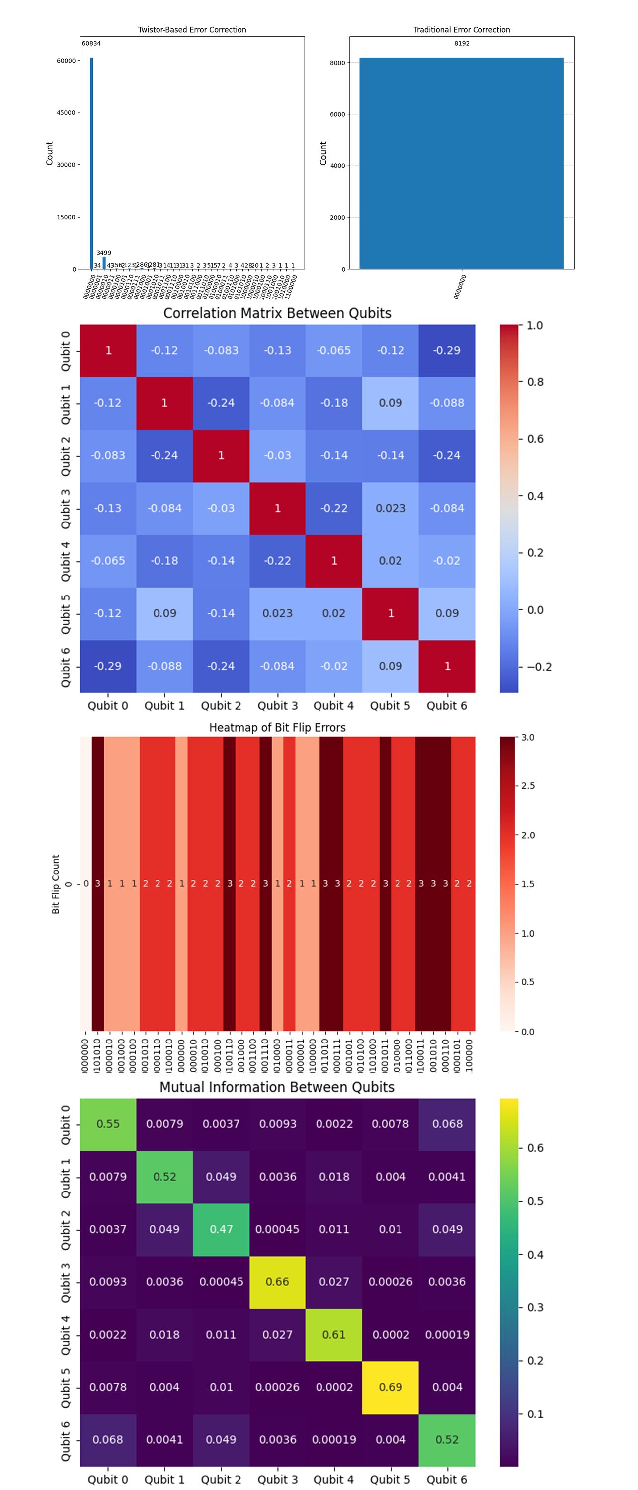
The classical fidelity calculation above (visual 1) (code below), as calculated using the Jensen-Shannon divergence approach, is ~ 0.9745. This shows that the probability distributions of the measurement outcomes from the twistor-based and traditional error correction schemes are quite similar, with a high degree of overlap. The closer the fidelity is to 1, the more similar the two distributions are.
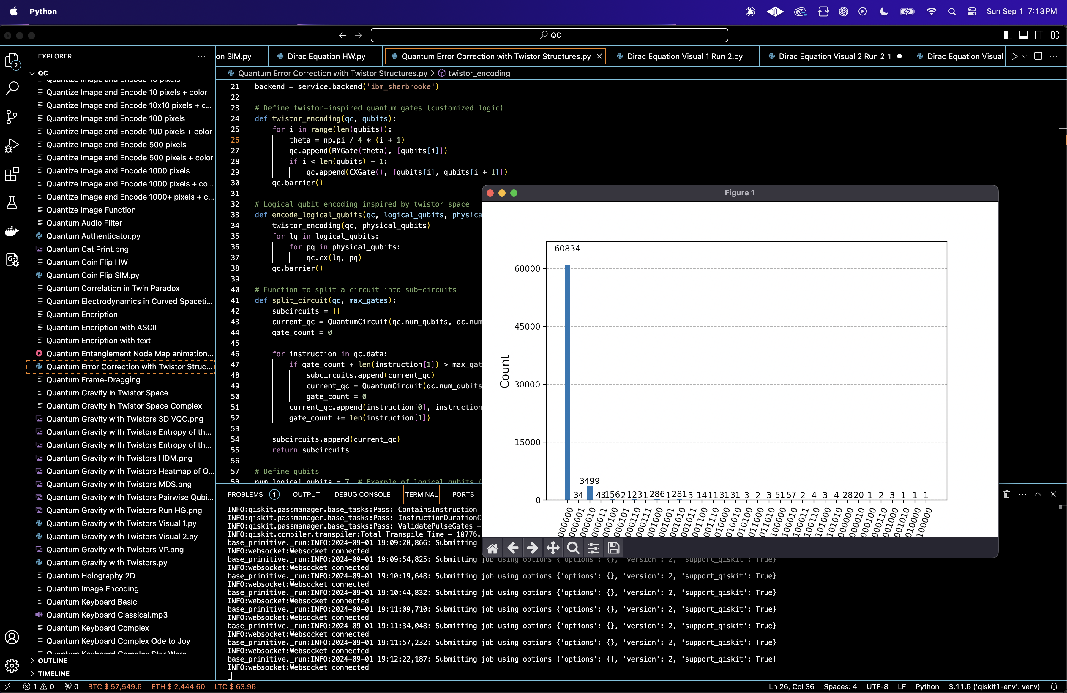
The histogram for the twistor-based scheme shows a significant concentration of measurements in the state '0000000', with 60,834 counts, indicating that the circuit effectively corrected most errors and returned the system to the expected state. There is also a noticeable spread across other states, with the next highest count being 3,499 in the '0000010' state, followed by several other states with lower but non-negligible counts. This spread suggests that while the twistor-based encoding was effective, it also introduced some noise or errors that were not entirely corrected. The histogram for the traditional error correction scheme shows a nearly perfect concentration of measurements in the '0000000' state, with all 8192 counts in that state. This indicates that the traditional encoding was highly effective in correcting errors, with no noticeable spread across other states. The traditional error correction scheme appears to be more robust and effective in this setup. Despite this, the high classical fidelity indicates that the twistor-based scheme's performance is still very close to that of the traditional scheme, suggesting that twistor-based encoding can be a viable approach.
The correlation matrix between qubits above (visual 2) (code below) shows how errors in one qubit are correlated with errors in another. The values range from -0.29 to 1.0, indicating some level of both positive and negative correlations. Most correlations between qubits are relatively low (closer to zero), indicating that errors in individual qubits are largely independent. The mostly low correlations suggest that the error-correcting code is effectively isolating qubit errors, which is desirable in error correction. The presence of negative correlations could indicate that certain types of errors are mutually exclusive.
The Heatmap of Bit-Flip Errors above (visual 3) (code below) shows the number of bit flips between the observed states and the ideal state '0000000'. The bit flips are relatively uniformly distributed among 1, 2, and 3-bit flips, with very few states having no bit flips (which is expected given the observed high fidelity for 0000000). The most common errors involve 2 or 3-bit flips, which might indicate that the noise affecting the system typically affects multiple qubits simultaneously.
The Mutual Information Between Qubits heatmap above (visual 4) (code below) shows the mutual information between pairs of qubits, which measures how much information is shared between them. Qubit pairs (0, 0), (3, 3), (4, 4), and (5, 5) show high mutual information, indicating that these qubits share a significant amount of information internally (which is expected because they are correlated with themselves). Some pairs, like (3, 4) and (4, 5), have non-zero mutual information, suggesting there might be some correlation between their errors. This could be due to crosstalk. The low mutual information values between most qubits indicate that errors in individual qubits are relatively independent.
Winding Number (Topological Invariant): 1104 The winding number, 1104, is a topological invariant that reflects the 'twisting' or 'winding' of the geometric structure formed by the state vectors. A high winding number indicates a complex topological structure in the error landscape. This suggests that the error syndromes are not just randomly distributed but have an intricate structure. Twistor Theory often deals with complex, non-trivial topological structures. The high winding number could be indicative of a non-trivial topology in the quantum state space.

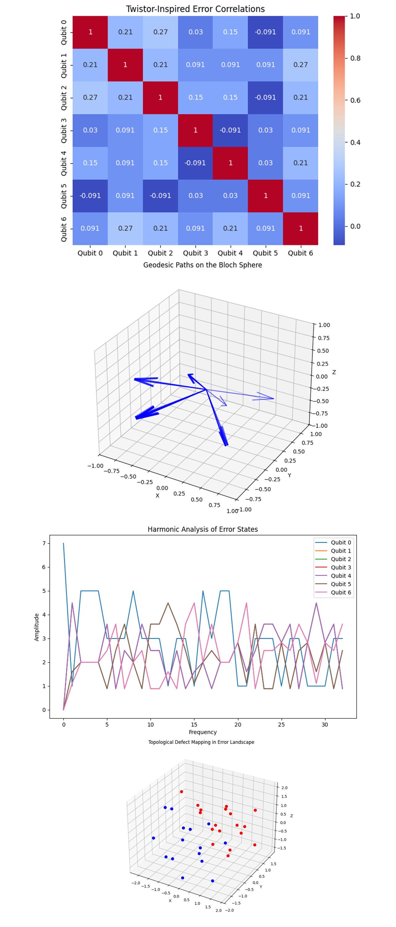
The heatmap of Twistor-Inspired Error Correlations above (visual 1) (code below) shows levels of correlation between qubits.
The presence of moderate correlations between certain qubit pairs indicates that these qubits are not entirely independent and could be influenced by shared crosstalk.
In Twistor Theory, correlations between different elements can reflect underlying geometric connections. The observed correlations may suggest that certain qubits are part of a structure within the twistor space that makes them more susceptible to correlated errors.
The geodesic paths on the Bloch Sphere visual above (visual 2) (code below) represents the evolution of qubit states in the Bloch sphere. In twistor theory, these paths might correspond to the most natural error correction trajectories that preserve certain topological features. The relatively short and direct paths suggest minimal error evolution, indicating that the qubits remain close to their intended states. Twistor-inspired approaches could leverage these paths to optimize error correction by maintaining the qubits along the most stable trajectories.
In the Harmonic Analysis of Error States visual above (visual 3) (code below), the Fourier transform reveals the frequency components of the error states. Peaks in the harmonic analysis suggest periodic errors, which could be indicative of systematic noise or recurring errors.
In the Topological Defect Mapping in Error Landscape above (visual 4) (code below), the red and blue points in 3D space represent distinct topological defects in the error landscape. The clustering of points indicates regions with higher concentrations of defects. In twistor theory, such defects correspond to singularities or disruptions in the twistor space. The spatial distribution suggests that certain regions of twistor space are more susceptible to these defects, which could be critical zones where quantum errors manifest.

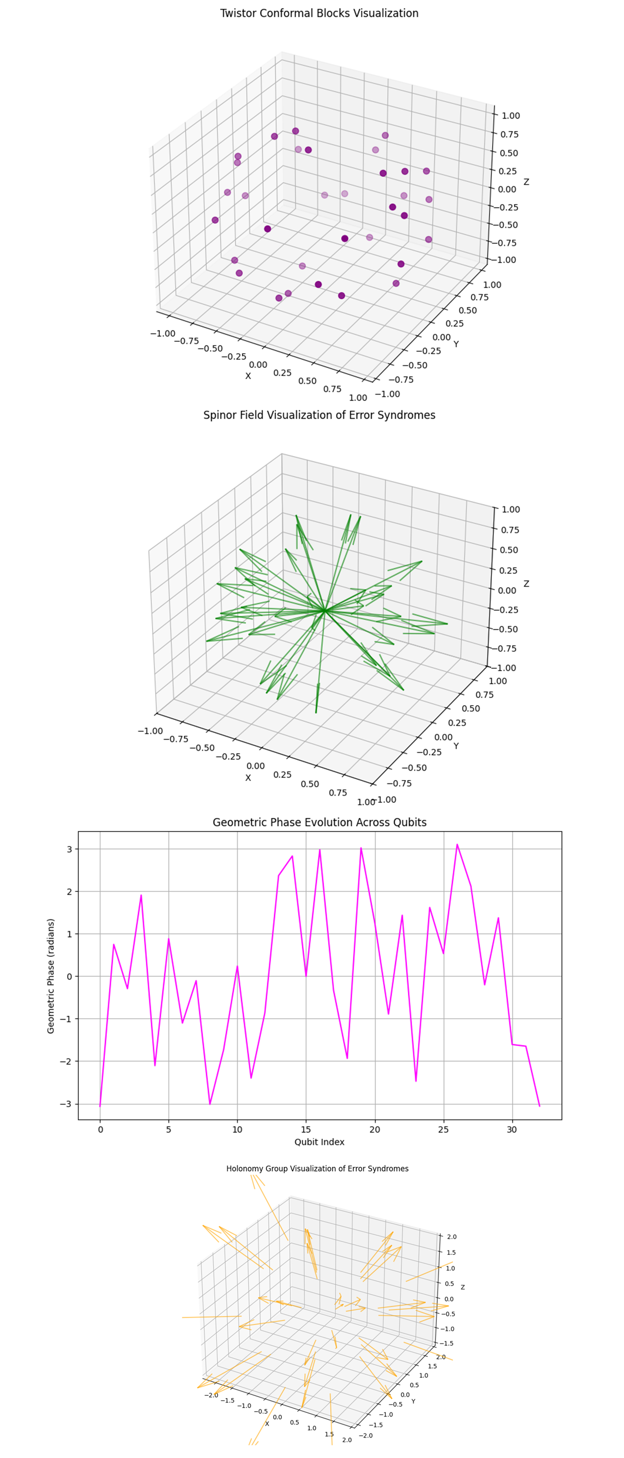
In the Twistor Conformal Blocks Visualization above (visual 1) (code below), the plot shows a distribution of points with varying intensity levels, representing how error syndromes map under conformal transformations. Twistor theory involves conformal transformations, which preserve angles but can distort other properties like distances. The variation in intensity suggests that error syndromes respond differently to these transformations. Regions of higher intensity indicate areas where errors might be less influenced by the twistor geometry, while lower intensities suggest regions where the twistor space has a stronger influence on the error structure.
In the Spinor Field Visualization of Error Syndromes above (visual 2) (code below), we see a 3D vector field with arrows representing the spinor form of the error states. The vectors in this plot reveal how spinors are aligned in the twistor space. Patterns in the alignment and direction of these spinors indicate correlations between error states that are inherent to the underlying twistor structure.
In the Geometric Phase Evolution Across Qubits visual above (visual 3) (code below), we see a plot showing significant variations in the geometric phase across different qubits. Geometric phases are closely related to the curvature and structure of twistor space. The observed fluctuations indicate that the qubits experience varying phase shifts, which are linked to the underlying geometry of the twistor space. These variations highlight how the twistor space influences the quantum system's phase evolution.
In the Holonomy Group Visualization of Error Syndromes visual above (visual 4) (code below), the 3D vectors represent the holonomy or how error vectors change under parallel transport in the error landscape. In twistor theory, holonomy groups describe the curvature of the space and how it affects parallel transport. The arrangement and direction of these vectors indicate how the error syndromes are altered when moved around loops in the twistor space. These changes reveal the twistor space's curvature properties and how they influence the stability and behavior of quantum errors.
In the end, this experiment explored a novel twistor-inspired quantum error correction scheme and compared its performance against a traditional error correction method. The results showed a Classical fidelity (Jensen-Shannon-based) of 0.974 for the twistor-based scheme, indicating a high degree of similarity between the twistor-corrected states and the traditional encoding. The histogram of measurement outcomes for the twistor-based scheme revealed that the dominant state accounted for the majority of the counts, with significant leakage into other states, while the traditional scheme showed a single dominant state.
The correlation matrix between qubits and the heatmap of Bit-Flip Errors revealed the degree of interaction and error propagation across the qubits, highlighting areas where errors were more likely to occur. The Mutual Information Between Qubits heatmap and Twistor-Inspired Error Correlations heatmap showed how data was shared and correlated between different qubits under the twistor-based encoding. The geodesic paths on the Bloch Sphere and Harmonic Analysis of Error States provided geometric and spectral insights into the behavior of qubits during the experiment. The Topological Defect Mapping in the Error Landscape and Twistor Conformal Blocks Visualization allowed us to identify and characterize topological features in the error syndromes, while the Spinor Field Visualization and Holonomy Group Visualization illustrated the evolution of spinor fields and holonomy groups. The experiment demonstrated the potential of twistor theory as a foundation for developing working quantum error correction schemes.
Code:
# imports
import numpy as np
from qiskit import QuantumCircuit, transpile
from qiskit_ibm_runtime import QiskitRuntimeService, Session, SamplerV2
from qiskit.visualization import plot_histogram
from qiskit_aer.noise import NoiseModel, depolarizing_error, amplitude_damping_error, coherent_unitary_error
from qiskit.circuit.library import RYGate, CXGate, HGate, CZGate  # Import necessary gates
import json
import logging
import matplotlib.pyplot as plt

# Setup logging
logging.basicConfig(level=logging. INFO)
logger = logging.getLogger(__name__)

# Load IBMQ account
service = QiskitRuntimeService(
    channel='ibm_quantum',
    instance='ibm-q/open/main',
    token='YOUR_IBMQ_KEY_O-`'
)
backend = service.backend('ibm_kyiv')

#  Twistor-inspired quantum gates
def twistor_encoding(qc, qubits):
    for i in range(len(qubits)):
        theta = np.pi / 4 * (i + 1)
        qc.append(RYGate(theta), [qubits[i]])
        if i < len(qubits) - 1:
            qc.append(CXGate(), [qubits[i], qubits[i + 1]])
    qc.barrier()

# Twistor-inspired Logical qubit encoding
def encode_logical_qubits(qc, logical_qubits, physical_qubits):
    twistor_encoding(qc, physical_qubits)
    for lq in logical_qubits:
        for pq in physical_qubits:
            qc. cx(lq, pq)
    qc.barrier()

# Function to split a circuit into sub-circuits
def split_circuit(qc, max_gates):
    subcircuits = []
    current_qc = QuantumCircuit(qc.num_qubits, qc.num_clbits)
    gate_count = 0

    for instruction in qc. data:
        if gate_count + len(instruction[1]) > max_gates:
            subcircuits.append(current_qc)
            current_qc = QuantumCircuit(qc.num_qubits, qc.num_clbits)
            gate_count = 0
        current_qc.append(instruction[0], instruction[1], instruction[2])
        gate_count += len(instruction[1])

    subcircuits.append(current_qc)
    return subcircuits

# Define qubits
num_logical_qubits = 7
num_physical_qubits = 127

logical_qubits = list(range(num_logical_qubits))
physical_qubits = list(range(num_logical_qubits, num_physical_qubits))

# Initialize quantum circuit
qc = QuantumCircuit(num_physical_qubits, num_logical_qubits)

# Twistor-inspired encoding logical qubits into physical
encode_logical_qubits(qc, logical_qubits, physical_qubits)

# Apply Hadamard gates to logical qubits (for state superposition)
for lq in logical_qubits:
    qc.h(lq)

# Introduce deliberate errors for testing purposes
qc. cx(logical_qubits[0], physical_qubits[10])
qc.x(physical_qubits[20])
qc. cz(physical_qubits[5], logical_qubits[1])

# Apply twistor encoding again to reinforce the encoding
twistor_encoding(qc, physical_qubits)

# Measure the logical qubits
qc.measure(logical_qubits, range(num_logical_qubits))

# Transpile the circuit
transpiled_qc = transpile(qc, backend=backend, optimization_level=3)

# Manually set a gate limit
max_gates = 5000

# Split the circuit into sub-circuits
subcircuits = split_circuit(transpiled_qc, max_gates)

# Run each sub-circuit on the backend and collect results
all_counts = {}
with Session(service=service, backend=backend) as session:
    sampler = SamplerV2(session=session)

    for idx, sub_qc in enumerate(subcircuits):
        job = sampler. run([sub_qc], shots=8192)
        job_result = job.result()

        # Retrieve the classical register name
        classical_register = sub_qc.cregs[0].name

        # Extract counts for the first (and only) pub result
        pub_result = job_result[0].data[classical_register].get_counts()

        # Combine the results
        for key, value in pub_result.items():
            if key in all_counts:
                all_counts[key] += value
            else:
                all_counts[key] = value

# Save the combined results
results_data = {
    "raw_counts": all_counts
}
file_path = '/Users/Documents/twistor_error_correction_results.json'
with open(file_path, 'w') as f:
    json.dump(results_data, f, indent=4)

# Visualize the combined results
plot_histogram(all_counts)
plt. show()

///////////////////////////////////////////////////////////////////////

Code that computes the classical fidelity between the Twistor-based and Traditional Error Correction results using Jensen-Shannon divergence
# imports
import numpy as np
from qiskit import QuantumCircuit, transpile
from qiskit_ibm_runtime import QiskitRuntimeService, Session, SamplerV2
from qiskit.visualization import plot_histogram
import json
import logging
import matplotlib.pyplot as plt
from scipy.spatial.distance import jensenshannon

# Logging
logging.basicConfig(level=logging. INFO)
logger = logging.getLogger(__name__)

# Load IBMQ account
service = QiskitRuntimeService(
    channel='ibm_quantum',
    instance='ibm-q/open/main',
    token='YOUR_IBMQ_KEY_O-`'
)
backend = service.backend('ibm_kyiv')

# Load twistor error correction results from JSON
twistor_file_path = '/Users/Documents/twistor_error_correction_results.json'
with open(twistor_file_path, 'r') as f:
    twistor_counts = json.load(f)['raw_counts']

# Define qubits
num_logical_qubits = 7  # Example of logical qubits (can be adjusted)
num_physical_qubits = 127

logical_qubits = list(range(num_logical_qubits))
physical_qubits = list(range(num_logical_qubits, num_physical_qubits))

# Initialize traditional quantum circuit
qc_traditional = QuantumCircuit(num_physical_qubits, num_logical_qubits)

# Traditional encoding scheme (Steane code)
def encode_logical_qubits_traditional(qc, logical_qubits, physical_qubits):
    for lq in logical_qubits:
        qc.h(lq)
        qc. cx(lq, physical_qubits[lq])
    qc.barrier()

encode_logical_qubits_traditional(qc_traditional, logical_qubits, physical_qubits)

# Transpile the traditional circuit
transpiled_qc_traditional = transpile(qc_traditional, backend=backend, optimization_level=3)

# Run the traditional circuit
with Session(service=service, backend=backend) as session:
    sampler = SamplerV2(session=session)

    job_traditional = sampler. run([transpiled_qc_traditional], shots=8192)
    job_result_traditional = job_traditional.result()

    # Get the traditional results
    classical_register_traditional = qc_traditional.cregs[0].name
    counts_traditional = job_result_traditional[0].data[classical_register_traditional].get_counts()

# Save the traditional results
traditional_file_path = '/Users/Documents/traditional_error_correction_results.json'
with open(traditional_file_path, 'w') as f:
    json.dump(counts_traditional, f, indent=4)

# Normalize counts to probability distribution
def normalize_counts(counts, shots):
    return {state: count / shots for state, count in counts.items()}

# Normalize the count distributions
total_shots = 8192
twistor_probs = normalize_counts(twistor_counts, total_shots)
traditional_probs = normalize_counts(counts_traditional, total_shots)

# Calculate Jensen-Shannon divergence fidelity
all_states = set(twistor_probs.keys()).union(set(traditional_probs.keys()))
twistor_vector = np.array([twistor_probs.get(state, 0) for state in all_states])
traditional_vector = np.array([traditional_probs.get(state, 0) for state in all_states])

# Compute the Jensen-Shannon divergence
js_divergence = jensenshannon(twistor_vector, traditional_vector)
classical_fidelity = 1 - js_divergence ** 2

# Logging the results
logger. info(f'Classical fidelity (Jensen-Shannon-based): {classical_fidelity}')

# Visualize the comparison of results
fig, axs = plt.subplots(1, 2, figsize=(14, 5))

# Plot the twistor-based histogram
axs[0].set_title('Twistor-Based Error Correction')
plot_histogram(twistor_counts, ax=axs[0])

# Plot the traditional histogram
axs[1].set_title('Traditional Error Correction')
plot_histogram(counts_traditional, ax=axs[1])

plt. show()

# End.
