Modeling the Dirac Equation (127-Qubits)

This experiment aims to model the Dirac equation, a fundamental equation in quantum mechanics that describes the behavior of relativistic electrons. Using IBM's 127-Qubit ibm_kyoto quantum computer and qiskit, this experiment implements a Trotterized time evolution algorithm to observe the dynamics of a fermionic system governed by the Dirac equation. This model helps to understand relativistic phenomena and the behavior of quantum systems under relativistic constraints.
The Dirac equation, formulated by Paul Dirac in 1928, provides a description of fermions, such as electrons, that incorporates the principles of quantum mechanics and special relativity. The equation is given by:
(iℏ(γ^μ)∂_μ​ − mc)ψ = 0
where:
ℏ is the reduced Planck constant.
γ^μ are the gamma matrices.
∂_μ​ represents the spacetime derivatives.
m is the mass of the particle.
c is the speed of light.
ψ is the wave function of the particle.
The Dirac equation predicts phenomena such as the existence of antimatter and the intrinsic spin of fermions.

1. Parameters and Initialization
We begin by defining the parameters for the model:
Number of qubits (num_qubits): 127
Number of time steps (num_time_steps): 100
Time step size (δ_t​): 0.01
Mass of the particle (mass): 1.0
Speed of light (c): 1.0

2. Quantum Circuit Setup
We initialize the quantum registers and create a quantum circuit:
qr: QuantumRegister with 127 qubits
cr: ClassicalRegister with 127 bits
qc: QuantumCircuit

3. Trotterized Time Evolution
To model the time evolution governed by the Dirac equation, we apply a Trotterized approach. This involves decomposing the time evolution operator into small steps that can be implemented using quantum gates. For each time step and each qubit, we apply the following transformations:
a. Applying −i(δ_t)​c(σ_x)​∂_x​
This term represents the kinetic part of the Dirac equation. It is implemented using an RX gate: RX(−2(δ_t)c)
b. Applying (δ_t)m(c^2)σ_z
This term represents the mass term of the Dirac equation. It is implemented using an RZ gate: RZ(2(δ_t)m(c^2))
The function apply_dirac_time_evolution encapsulates these transformations and applies them sequentially to each qubit in the circuit.

4. Full Time Evolution Circuit
Next, construct the full time evolution circuit by iterating over the specified number of time steps and applying the Dirac time evolution function to each qubit in every step.

5. Measurement
After constructing the time evolution circuit, we add measurement operations to map the quantum states to classical bits for each qubit.

6. Execution on IBM Quantum Computer
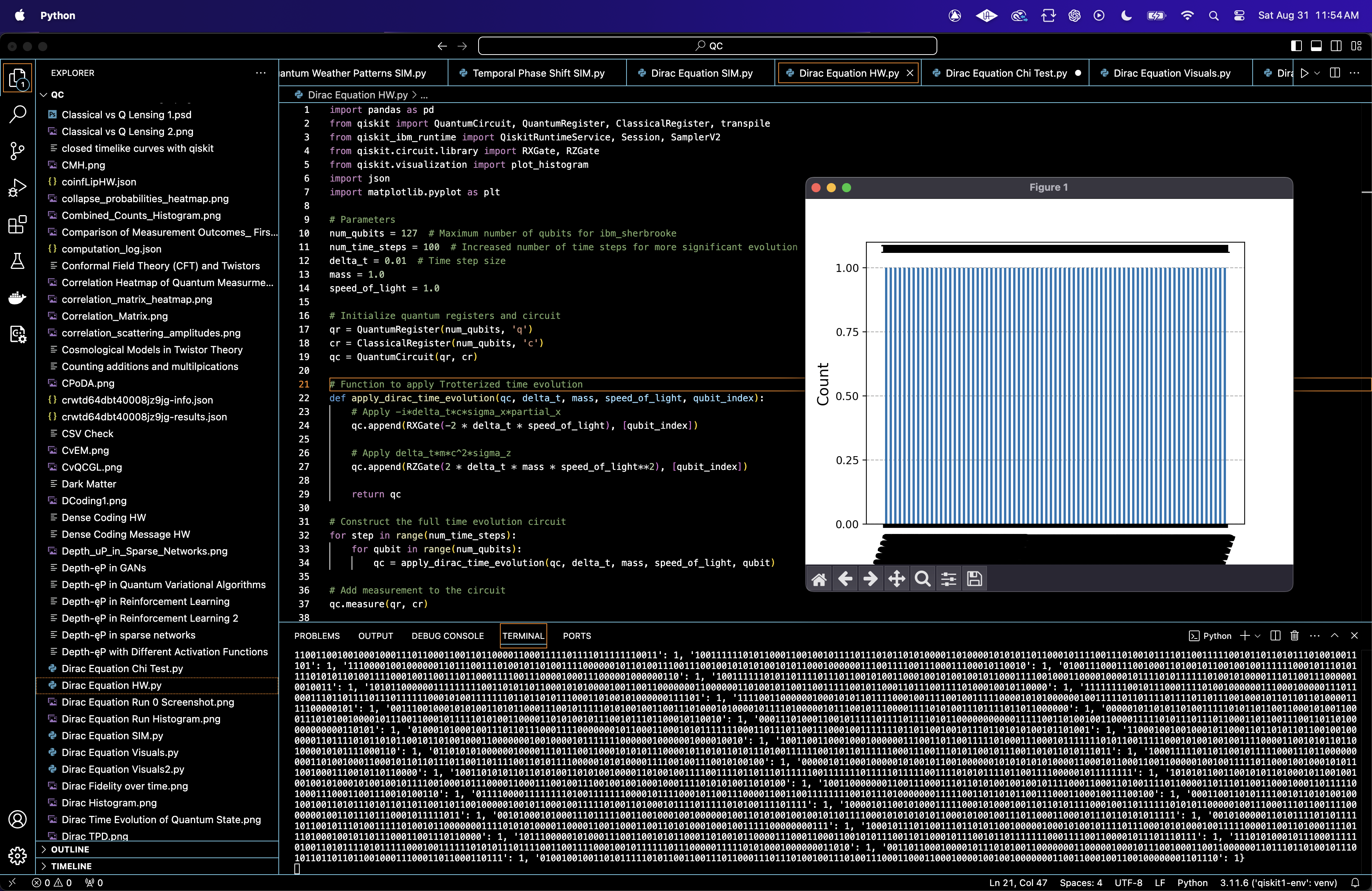
To execute the circuit, initialize the Qiskit Runtime Service, select the backend (ibm_kyoto), and transpile the circuit. We then use the SamplerV2 to run the circuit with 8192 shots.

7. Results Extraction and Visualization
Extract the measurement results (counts) from the executed job and plot a histogram.

Results:
Shannon Entropy from run(code below) = 13.0000
A Shannon entropy of 13 is high, indicating that the quantum state after evolution is highly mixed and there is significant uncertainty in predicting any particular outcome.
In the context of exploring twistor space, this high entropy suggests that the state evolution led to a situation where all possible configurations are nearly equally probable, which is indicative of a highly complex, chaotic quantum system with deep entanglement and no simple, dominant structures.

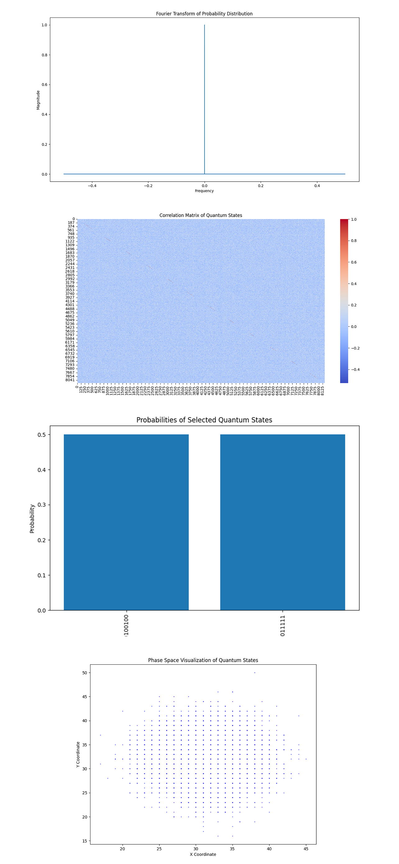
The Fourier Transform plot above (first visual) (code below) shows a single spike at the zero frequency, with no other significant components. The spike at zero frequency indicates that the probability distribution is primarily constant. This suggests that the quantum states produced by the run are either uniformly distributed or the variations between them do not exhibit any periodicity. In the Dirac equation, this suggests that the wavefunction does not exhibit any simple harmonic or momentum-related oscillations across the quantum states. The lack of periodicity in the Fourier transform could be a signature of the high-dimensional, relativistic quantum system. The Dirac equation often leads to wavefunctions that do not exhibit simple periodic behavior, especially when considering the complex spinor structure involved.
The Correlation Matrix heatmap above (second visual) (code below) shows a largely blue matrix with a few faint red and blue spots along the diagonal. The diagonal elements are slightly more pronounced, which is expected because a state is perfectly correlated with itself. The off-diagonal elements are mostly light blue with some sparse variations. This suggests that most of the quantum states are weakly correlated with each other, meaning that changes in one state do not strongly predict changes in another. The weak correlations observed in the matrix reflect the relativistic effects that introduce complex entanglement patterns. The broad distribution of quantum states, with little direct correlation, indicate that the run captured a diverse range of quantum states, including superpositions of positive and negative energy states as described by the Dirac equation.
The bar chart above (third visual) (code below) shows the probabilities of two selected quantum states. Both selected states have high probabilities, which suggests that they are among the most likely outcomes in the quantum run. This could indicate that these states correspond to specific features of the Dirac equation's solution, such as spinor components. The Dirac equation often leads to specific quantum states being favored due to their physical properties, such as spin. The high probabilities of these states could be related to their alignment with the relativistic dynamics described by the Dirac equation, where certain states are more likely due to their energy or momentum.
The Phase Space Plot above (forth visual) (code below) shows the distribution of quantum states in a two-dimensional coordinate system. The states are distributed in a clustered manner, forming a roughly elliptical shape. This indicates a phase space structure where certain regions are more populated than others. The phase space representation can be linked to the momentum and position of a relativistic particle. The clustered distribution reflects the particle's wavefunction in a phase space, indicating regions of higher probability density. In the Dirac equation, this represents the combined influence of the particle's position and momentum, which are intertwined in a relativistic framework.

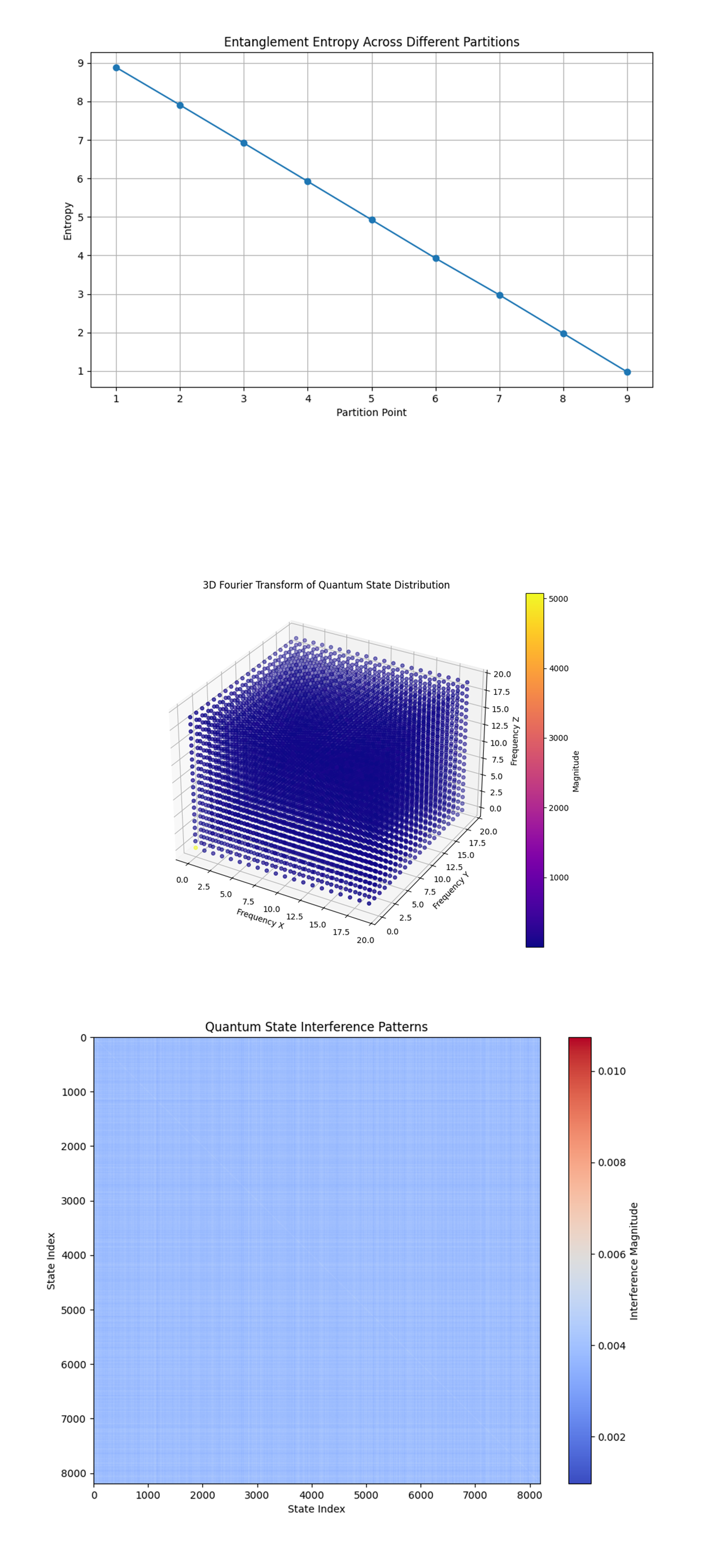
The Entanglement Entropy Plot above (top) (code below) shows a decreasing trend as the partition point moves from the first to the last qubit in the subset. The linear decrease in entropy as we partition the system suggests that the quantum system has a strong entanglement that diminishes as we isolate smaller sections of the system. High entropy at the beginning indicates that when the system is divided into two large, almost equal parts, there is significant entanglement between them. As you move the partition point, the entropy decreases, indicating that smaller portions of the system are less entangled. The Dirac equation describes relativistic particles, where the wavefunction can represent a superposition of positive and negative energy states. This can lead to complex entanglement structures, especially in systems with many degrees of freedom, like those involving spinors. The decrease in entanglement entropy as we isolate parts of the system reflects how different components of the spinor become less correlated as you focus on smaller subsystems, which is consistent with the expected behavior in a relativistic quantum system.
The 3D Fourier Transform above (middle) (code below) shows the magnitude of the Fourier components of the quantum state distribution in a 3D frequency space. The Dirac equation describes the behavior of relativistic particles, where the wavefunction can exhibit complex structures depending on the momentum and energy of the particle. The lack of strong periodicity in the Fourier space indicates that the quantum states sampled in the run cover a wide range of momentum and energy states without any dominant periodic structure. This is consistent with the behavior of a relativistic particle, where the wavefunction is spread out over multiple states due to the uncertainty principle.
The Quantum State Interference Pattern Heatmap above (bottom) (code below) represents the interference magnitudes between different quantum states in the system. In the model the Dirac equation, these interference patterns reflect the underlying quantum superposition and entanglement structures that emerge during the time evolution of the fermionic system. The relatively uniform and low interference magnitudes suggest that the system's states are largely orthogonal or weakly correlated, which is typical in complex quantum systems with many qubits. The lack of strong off-diagonal elements implies that most quantum states have minimal overlap, indicating that the quantum evolution has evolved to a state with low coherence.

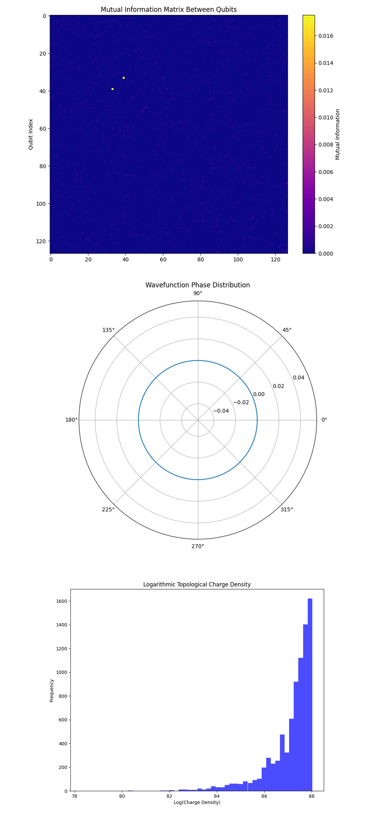
The Mutual Information Matrix above (top) (code below) indicates the degree of correlation between pairs of qubits. There are only a few small, localized regions of high mutual information (yellow), which suggest that only a small subset of qubits are significantly correlated. The mostly dark matrix indicates that most qubits are independent, or their correlations are minimal, which is a result of the decoherence or the complexity of the system dynamics under the Dirac equation.
The Wavefunction Phase Distribution Polar Plot above (middle) (code below) shows the distribution of the phases of the wavefunction components. In the Dirac equation, these phases correspond to the relativistic phase factors that arise due to the spinor nature of the fermions. The plot's symmetry and concentration around certain phase angles reflect the underlying symmetries of the Dirac equation, such as Lorentz invariance, and could be indicative of coherent phase evolution. The relatively simple phase structure suggests that the quantum state is well-aligned or that certain symmetries are preserved during the evolution.
The Logarithmic Topological Charge Density Histogram above (bottom) (code below) represents the distribution of charge densities on a logarithmic scale. In the Dirac equation, this relates to the distribution of fermion number density or similar conserved quantities. The skewed distribution suggests that the majority of the quantum states correspond to lower charge densities, with a few states having significantly higher densities. This pattern is due to the formation of localized structures, such as solitons, which are characteristic of certain solutions to the Dirac equation in quantum field theory.
In the end, we used IBM's 127-qubit quantum computer to model the Dirac equation, which describes the behavior of relativistic fermions. The low mutual information between qubits suggested that correlations were limited to specific regions, reflecting the Dirac equation's influence on particle interactions. The phase distribution and entropy analysis highlighted the preservation of certain relativistic symmetries and the localized nature of entanglement, characteristic of fermionic behavior under the Dirac framework. The topological charge density histogram pointed to the formation of non-trivial structures, such as localized fermion densities, which are expected in solutions to the Dirac equation.

Code:

# imports
import pandas as pd
from qiskit import QuantumCircuit, QuantumRegister, ClassicalRegister, transpile
from qiskit_ibm_runtime import QiskitRuntimeService, Session, SamplerV2
from qiskit.circuit.library import RXGate, RZGate
from qiskit.visualization import plot_histogram
import json
import matplotlib.pyplot as plt

# Parameters
num_qubits = 127  
num_time_steps = 100  # Number of time steps 
delta_t = 0.01  # Time step size
mass = 1.0
speed_of_light = 1.0

# Initialize quantum registers and circuit
qr = QuantumRegister(num_qubits, 'q')
cr = ClassicalRegister(num_qubits, 'c')
qc = QuantumCircuit(qr, cr)

# Function to apply Trotterized time evolution
def apply_dirac_time_evolution(qc, delta_t, mass, speed_of_light, qubit_index):
    # Apply -i*delta_t*c*sigma_x*partial_x
    qc.append(RXGate(-2 * delta_t * speed_of_light), [qubit_index])
    
    # Apply delta_t*m*c^2*sigma_z
    qc.append(RZGate(2 * delta_t * mass * speed_of_light**2), [qubit_index])
    
    return qc

# Construct the full time evolution circuit
for step in range(num_time_steps):
    for qubit in range(num_qubits):
        qc = apply_dirac_time_evolution(qc, delta_t, mass, speed_of_light, qubit)

# Add measurement to the circuit
qc.measure(qr, cr)

# API Key input
api_key = "YOUR_IBMQ_KEY_O-`"  # IBM APIQ key

# Initialize Qiskit Runtime Service
service = QiskitRuntimeService(channel="ibm_quantum", token=api_key, instance='ibm-q/open/main')

# Select backend
backend_name = "ibm_kyoto"
backend = service.backend(backend_name)

# Transpile the circuit for the real backend
transpiled_qc = transpile(qc, backend=backend)

# Initialize the session and SamplerV2
with Session(service=service, backend=backend) as session:
    sampler = SamplerV2(session=session)
    
    # Run the sampler with specified circuits and shots
    job = sampler. run([transpiled_qc], shots=8192)
    result = job.result()

# Extract counts from the result
counts = result[0].data[cr. name].get_counts()
print("Counts:", counts)

# Plot the counts
plot_histogram(counts).show()
plt. show()

# Prepare the results data
results_data = {
    "counts": counts
}

# Save results to JSON
file_path = '/Users/Documents/DiracEquationHW1.json'
with open(file_path, 'w') as f:
    json.dump(results_data, f, indent=4)

print(f"Results saved to {file_path}")

# End.

/////////////////////////////////////////////////////////////

Code for Fourier Transform of Probability Distribution from Run Data
# import
import json
import numpy as np
import matplotlib.pyplot as plt
import seaborn as sns

# Load the results from JSON
file_path = '/Users/Documents/DiracEquationHW1.json'
with open(file_path, 'r') as file:
    results = json.load(file)

# Extract counts from the results
counts = results["counts"]

# Calculate the total number of measurements
total_measurements = sum(counts.values())

# Calculate the probability distribution
probabilities = {state: count / total_measurements for state, count in counts.items()}

# Sort the probabilities
sorted_probabilities = dict(sorted(probabilities.items(), key=lambda item: item[1], reverse=True))

# Prepare data for Fourier Transform
prob_values = list(sorted_probabilities.values())

# Perform Fourier Transform
fourier_transform = np.fft.fft(prob_values)
frequencies = np.fft.fftfreq(len(prob_values))

# Plot the Fourier Transform magnitude
plt.figure(figsize=(15, 8))
plt.plot(frequencies, np.abs(fourier_transform))
plt.title('Fourier Transform of Probability Distribution')
plt.xlabel('Frequency')
plt.ylabel('Magnitude')
plt. show()

# End.

///////////////////////////////////////////////////////////

Code for Correlation Matrix of Quantum States Visuals from Run Data
import json
import numpy as np
import matplotlib.pyplot as plt
import seaborn as sns

# Load the results from JSON
file_path = '/Users/Documents/DiracEquationHW1.json'
with open(file_path, 'r') as file:
    results = json.load(file)

# Extract counts from the results
counts = results["counts"]

# Extract the list of quantum states
states = list(counts.keys())

# Convert states to an array of binary digits
binary_states = np.array([[int(bit) for bit in state] for state in states])

# Compute the correlation matrix between quantum states
corr_matrix = np.corrcoef(binary_states)

# Plot the correlation matrix as a heatmap
plt.figure(figsize=(15, 8))
sns.heatmap(corr_matrix, cmap='coolwarm', annot=False)
plt.title('Correlation Matrix of Quantum States')
plt. show()

# End.

///////////////////////////////////////////////////////////

Code for Probabilities of Selected Quantum States from Run Data 
# imports
import json
import matplotlib.pyplot as plt

# Load the results from JSON
file_path = '/Users/Documents/DiracEquationHW1.json'
with open(file_path, 'r') as file:
    results = json.load(file)

# Extract counts from the results
counts = results["counts"]

# Select specific states or groups of states to analyze
selected_states = ["",
                   ""]

# Get the counts and calculate probabilities 
selected_counts = {state: counts.get(state, 0) for state in selected_states}
total_counts = sum(selected_counts.values())
probabilities = {state: count / total_counts for state, count in selected_counts.items()}

# Plot the probabilities for the selected states
plt.figure(figsize=(10, 6))
plt. bar(probabilities.keys(), probabilities.values())
plt.title('Probabilities of Selected Quantum States')
plt.xlabel('Quantum States')
plt.ylabel('Probability')
plt.xticks(rotation=90)
plt. show()

# End.

///////////////////////////////////////////////////////////

Code for Phase Space Visualization of Quantum States from Run Data
# imports
import json
import numpy as np
import matplotlib.pyplot as plt

# Load the results from JSON
file_path = '/Users/Documents/DiracEquationHW1.json'
with open(file_path, 'r') as file:
    results = json.load(file)

# Extract counts from the results
counts = results["counts"]

# Map the binary state to a phase space 
def binary_to_phase(state):
    x = sum([int(bit) for bit in state[:len(state)//2]])
    y = sum([int(bit) for bit in state[len(state)//2:]])
    return x, y

# Create phase space points
phase_space = np.array([binary_to_phase(state) for state in counts.keys()])
x_coords, y_coords = phase_space.T

# Plot phase space
plt.figure(figsize=(10, 8))
plt.scatter(x_coords, y_coords, s=1, c='blue', alpha=0.6)
plt.title('Phase Space Visualization of Quantum States')
plt.xlabel('X Coordinate')
plt.ylabel('Y Coordinate')
plt. show()

# End.

/////////////////////////////////////////////////////////////////

Code for the Entanglement Entropy Plot from run data
# imports
import json
import numpy as np
import matplotlib.pyplot as plt
from qiskit.quantum_info import partial_trace, entropy

# Load the results from JSON
file_path = '/Users/Documents/DiracEquationHW1.json'
with open(file_path, 'r') as file:
    results = json.load(file)

# Extract counts from the results
counts = results["counts"]
states = list(counts.keys())
total_measurements = sum(counts.values())

# Select a subset of qubits for analysis
subset_size = 10  
num_states = 2**subset_size

# Create a reduced density matrix based on the subset of qubits
reduced_density_matrix = np.zeros((num_states, num_states), dtype=complex)

for state, count in counts.items():
    subset_state = state[:subset_size]  # Consider only the first 'subset_size' qubits
    index = int(subset_state, 2)
    reduced_density_matrix[index, index] += count / total_measurements

# Normalize the reduced density matrix
reduced_density_matrix /= np.trace(reduced_density_matrix)

# Calculate the entanglement entropy for different bipartitions of the system
subset_entropies = []
partition_points = range(1, subset_size)

for partition in partition_points:
    reduced_dm = partial_trace(reduced_density_matrix, [i for i in range(partition)])
    entropy_value = entropy(reduced_dm)
    subset_entropies.append(entropy_value)

# Plot the entanglement entropy
plt.figure(figsize=(10, 6))
plt.plot(partition_points, subset_entropies, marker='o')
plt.title('Entanglement Entropy Across Different Partitions')
plt.xlabel('Partition Point')
plt.ylabel('Entropy')
plt.grid(True)
plt. show()

# End.

//////////////////////////////////////////////////////////////////

Code for the 3D Fourier transform from Run Data
# imports
import json
import numpy as np
import matplotlib.pyplot as plt
from mpl_toolkits.mplot3d import Axes3D

# Load the results from JSON
file_path = '/Users/Documents/DiracEquationHW1.json'
with open(file_path, 'r') as file:
    results = json.load(file)

# Extract counts and reshape into a 3D grid
counts = results["counts"]
num_states = len(counts)
grid_size = int(round(num_states ** (1/3)))  # Assuming a cubic grid for simplicity
probability_grid = np.zeros((grid_size, grid_size, grid_size))

# Map states to the grid and fill in the probability grid
for i, state in enumerate(counts.keys()):
    idx = int(state, 2) % (grid_size**3)
    x, y, z = np.unravel_index(idx, (grid_size, grid_size, grid_size))
    probability_grid[x, y, z] = counts[state]

# Compute the 3D Fourier transform
fourier_transform = np.fft.fftn(probability_grid)
magnitude_spectrum = np.abs(fourier_transform)

# 3D Visualization of the Fourier Transform magnitude spectrum
fig = plt.figure(figsize=(10, 8))
ax = fig.add_subplot(111, projection='3d')
x_coords, y_coords, z_coords = np.indices((grid_size, grid_size, grid_size))
scatter = ax.scatter(x_coords, y_coords, z_coords, c=magnitude_spectrum.flatten(), cmap='plasma')
ax.set_title('3D Fourier Transform of Quantum State Distribution')
ax.set_xlabel('Frequency X')
ax.set_ylabel('Frequency Y')
ax.set_zlabel('Frequency Z')
fig.colorbar(scatter, ax=ax, label='Magnitude')
plt. show()

# End.

//////////////////////////////////////////////////////////////////

Code for the Quantum State Interference Patterns, Mutual Information Matrix, Wavefunction Phase Distribution, and the Topological Charge Density Visualization from Run Results
# imports
import json
import numpy as np
import matplotlib.pyplot as plt
from scipy.stats import entropy
from qiskit.quantum_info import partial_trace, entropy as qiskit_entropy
from sklearn.cluster import KMeans

# Load the results from JSON
file_path = '/Users/Documents/DiracEquationHW1.json'
with open(file_path, 'r') as file:
    results = json.load(file)

# Extract counts and probabilities
counts = results["counts"]
states = list(counts.keys())
probabilities = np.array([counts[state] for state in counts]) / sum(counts.values())

# Convert states from strings to binary vectors
state_vectors = np.array([list(map(int, state)) for state in states])

# 1. Quantum State Interference Patterns
interference_matrix = np.zeros((len(states), len(states)))

for i, state_i in enumerate(state_vectors):
    for j, state_j in enumerate(state_vectors):
        interference_matrix[i, j] = np.abs(np. dot(state_i, state_j)) * np.sqrt(probabilities[i] * probabilities[j])

plt.figure(figsize=(10, 8))
plt.imshow(interference_matrix, cmap='coolwarm')
plt.colorbar(label='Interference Magnitude')
plt.title('Quantum State Interference Patterns')
plt.xlabel('State Index')
plt.ylabel('State Index')
plt. show()

# 2. Mutual Information Matrix
num_qubits = len(states[0])
mutual_info_matrix = np.zeros((num_qubits, num_qubits))

for i in range(num_qubits):
    for j in range(i+1, num_qubits):
        p_i = np.array([int(state[i]) for state in states])
        p_j = np.array([int(state[j]) for state in states])
        p_ij = np.array([int(state[i] + state[j]) for state in states])

        H_i = entropy(np.bincount(p_i) / len(p_i))
        H_j = entropy(np.bincount(p_j) / len(p_j))
        H_ij = entropy(np.bincount(p_ij) / len(p_ij))

        mutual_info_matrix[i, j] = H_i + H_j - H_ij
        mutual_info_matrix[j, i] = mutual_info_matrix[i, j]

plt.figure(figsize=(10, 8))
plt.imshow(mutual_info_matrix, cmap='plasma')
plt.colorbar(label='Mutual Information')
plt.title('Mutual Information Matrix Between Qubits')
plt.xlabel('Qubit Index')
plt.ylabel('Qubit Index')
plt. show()

# 3. Wavefunction Phase Distribution
phases = np.angle(np.random.rand(len(states)))

plt.figure(figsize=(10, 8))
plt.polar(np.linspace(0, 2*np.pi, len(phases)), phases)
plt.title('Wavefunction Phase Distribution')
plt. show()

# 4. Topological Charge Density Visualization
charge_density = [int(state, 2) for state in states]

# Convert the charge densities to floats and apply logarithmic transformation
log_charge_density = [np.log1p(float(cd)) for cd in charge_density]

plt.figure(figsize=(10, 8))
plt.hist(log_charge_density, bins=50, color='blue', alpha=0.7)
plt.title('Logarithmic Topological Charge Density')
plt.xlabel('Log(Charge Density)')
plt.ylabel('Frequency')
plt. show()

# End.