Modeling Abstract Quantum Gravity Using Twistor Theory (127-Qubits)

This experiment aims to model aspects of abstract quantum gravity through twistor theory using IBM's 127-qubit ibm_kyoto and qiskit. The experiment constructs a quantum circuit that represents a twistor network, with each qubit acting as a twistor node. The circuit models the propagation of twistors through entanglement, introduces abstract quantum gravitational effects via parametrized rotation gates, and measures the resulting states.

1. Initialization of the Twistor Network
Initialize each qubit in a superposition state to model the quantum nature of twistors. In twistor theory, twistors are complex objects that can exist in multiple states simultaneously.
The initial state of each qubit is ∣0⟩. Applying the Hadamard gate H to each qubit puts it into a superposition:
H∣0⟩ = 1/sqrt(2) * ​(∣0⟩ + ∣1⟩)
This superposition state represents the twistor's ability to exist in multiple states.
We apply the Hadamard gate H to all 127 qubits in the circuit:
qc.h(qubit) for each qubit in the range 0 to 126

2. Entanglement to Model Twistor Propagation
We Model the propagation of twistors between nodes by introducing entanglement between pairs of qubits. In twistor theory, the connections between twistors are essential in defining their relationships and interactions.
Entanglement is achieved using the Controlled-Z gate (CZ). When applied to a pair of qubits, it creates a state where the two qubits are interdependent:
CZ(∣a⟩ ⊗ ∣b⟩) = (−1)^(ab) ∣a⟩ ⊗ ∣b⟩
where a and b are the states of the first and second qubits.
We apply the CZ gate between adjacent pairs of qubits:
qc. cz(qubit, qubit + 1) for qubits in the range 0 to 125

3. Simulating Abstract Quantum Gravitational Effects with Rotation Gates
Introduce abstract quantum gravitational effects by applying random rotations to each qubit. These rotations represent the influence of a quantum gravitational background on the twistor network, such as curvature.
The rotations around the X, Y, and Z axes are represented by the gates RX(θ_x), RY(θ_y), and RZ(θ_z), where θ_x​, θ_y, and θ_z​ are randomly chosen angles:
RX(θ_x​) = e^((−iθ_x * ​X)/2)
RY(θ_y​) = e^((−iθ_y​ * Y)/2)
RZ(θ_z​) = e^((−iθ_z​ * Z)/2)
For each qubit, we apply the rotation gates with random angles:
qc.rx(θ_x​, qubit)
qc.ry(θ_y​, qubit)
qc.rz(θ_z​, qubit) where θ_x​, θ_y​, θ_z​ ∼ Uniform(0, 2π)

4. Additional Entanglement to Model Complex Interactions
We introduce further entanglement between qubits to model more complex interactions within the twistor network, reflecting higher-order effects in quantum gravity.
The Controlled-X (CNOT) gate is used to create additional entanglement between qubits that are not directly adjacent:
CNOT(∣a⟩ ⊗ ∣b⟩) = ∣a⟩ ⊗ ∣ a ⊕ b⟩
where ⊕ denotes a XOR operation.
We apply the CNOT gate between every third qubit:
qc. cx(qubit, qubit + 2) for qubits in the range 0 to 124

5. Measurement of All Qubits
Measure the final state of each qubit to analyze the behavior of the twistor network under the influence of modeled quantum gravitational effects.
The measurement collapses each qubit into either ∣0⟩ or ∣1⟩, providing a classical bit for each qubit:
M(∣ψ⟩)= {
∣0⟩ with probability ∣⟨0 ∣ ψ⟩∣^2
∣1⟩​ with probability ∣⟨1 ∣ ψ⟩∣^2​
Measure all qubits and store the results in a classical register:
qc.measure(range(num_qubits), range(num_qubits))

6. Transpilation and Execution on IBM's ibm_kyoto
Optimize the quantum circuit for execution on ibm_kyoto.
Transpilation optimizes the quantum gates and their layout to reduce error rates and execution time:
qc → transpiled_qc = Transpile(qc, backend = ibm_kyoto, optimization_level = 3)
The transpiled circuit is then executed on the backend with 8192 shots (repetitions):
job = sampler. run([transpiled_qc], shots = 8192)

7. Analysis and Result Visualization
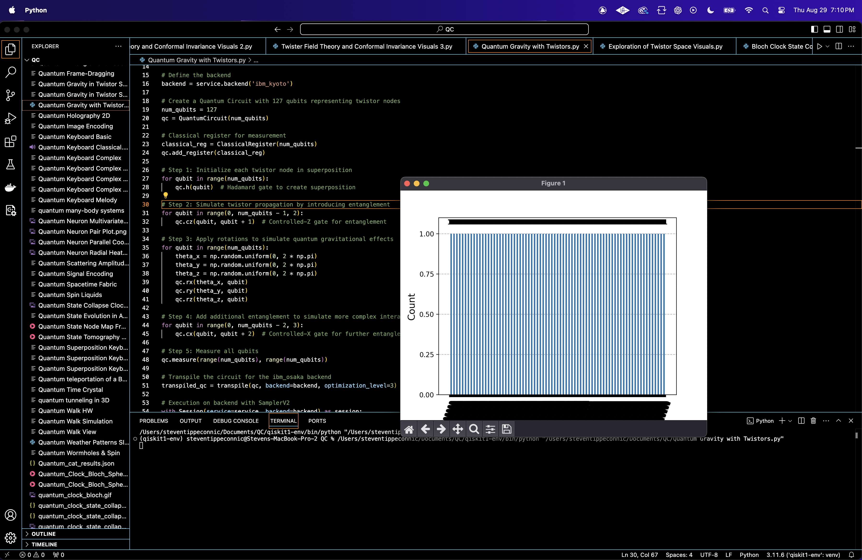
The counts of the measurement outcomes are extracted, and a histogram is plotted to visualize the distribution.
The measurement results are saved to a JSON.

Results:
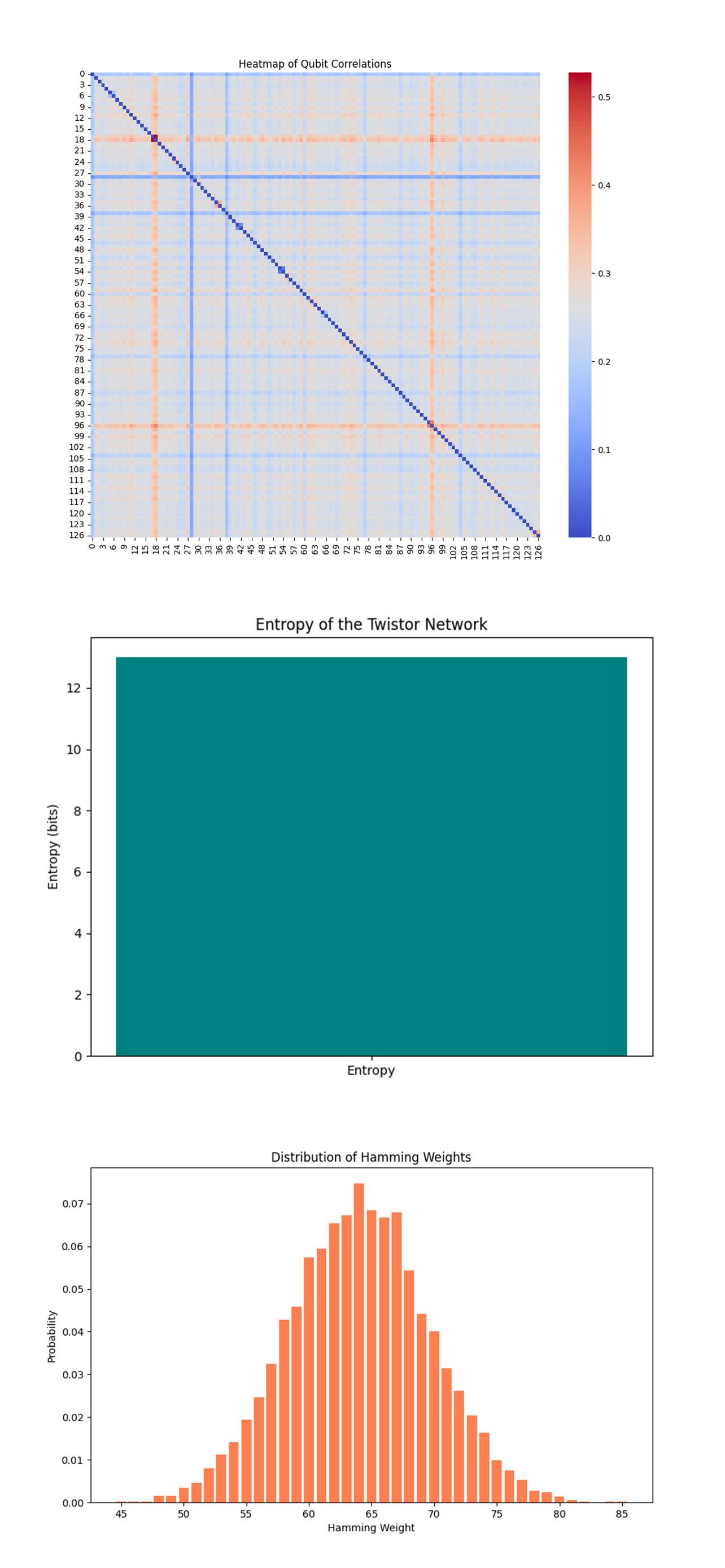
Shannon Entropy from run(code below) = 13.0000
A Shannon entropy of 13 is high, indicating that the quantum state after evolution is highly mixed and there is significant uncertainty in predicting any particular outcome.
In the context of exploring twistor space, this high entropy suggests that the state evolution led to a situation where all possible configurations are nearly equally probable, which is indicative of a highly complex, chaotic quantum system with deep entanglement and no simple, dominant structures.

The heatmap above (top) (code below) shows correlations between pairs of qubits, with both positive (red) and negative (blue) correlations present. The diagonal line represents self-correlations (each qubit with itself). There are notable off-diagonal patterns, suggesting that some qubits are strongly correlated or anti-correlated with others.
The presence of strong correlations between non-adjacent qubits suggests that the entangling gates in the circuit successfully created entanglement across the qubit network.
The negative correlations indicate anti-correlated behavior between specific pairs of qubits, which could be due to the abstract quantum gravitational perturbations in the circuit.
The entropy of the system was calculated to be 13 bits, which is the maximum possible for a 127-qubit system.
This high entropy indicates that the system is in a state of maximal disorder, where each outcome is equally probable, leading to no discernible order or pattern.
In the context of quantum gravity and twistors, suggesting that the modeled gravitational perturbations and entanglements have led to a highly complex state.
The Hamming weight distribution above (bottom) (code below) shows a clear bell-shaped curve, centered around a weight of 63-65. This indicates that most measurement outcomes have a nearly equal number of 0s and 1s.
The bell-shaped curve suggests that the system, despite its overall high entropy, exhibits some statistical regularity, with states having a roughly equal mix of 0s and 1s being the most probable.
This distribution is expected given the large number of qubits, where a uniform random distribution would naturally lead to most outcomes having a Hamming weight near the middle of the possible range (around 63-64 for 127 qubits).

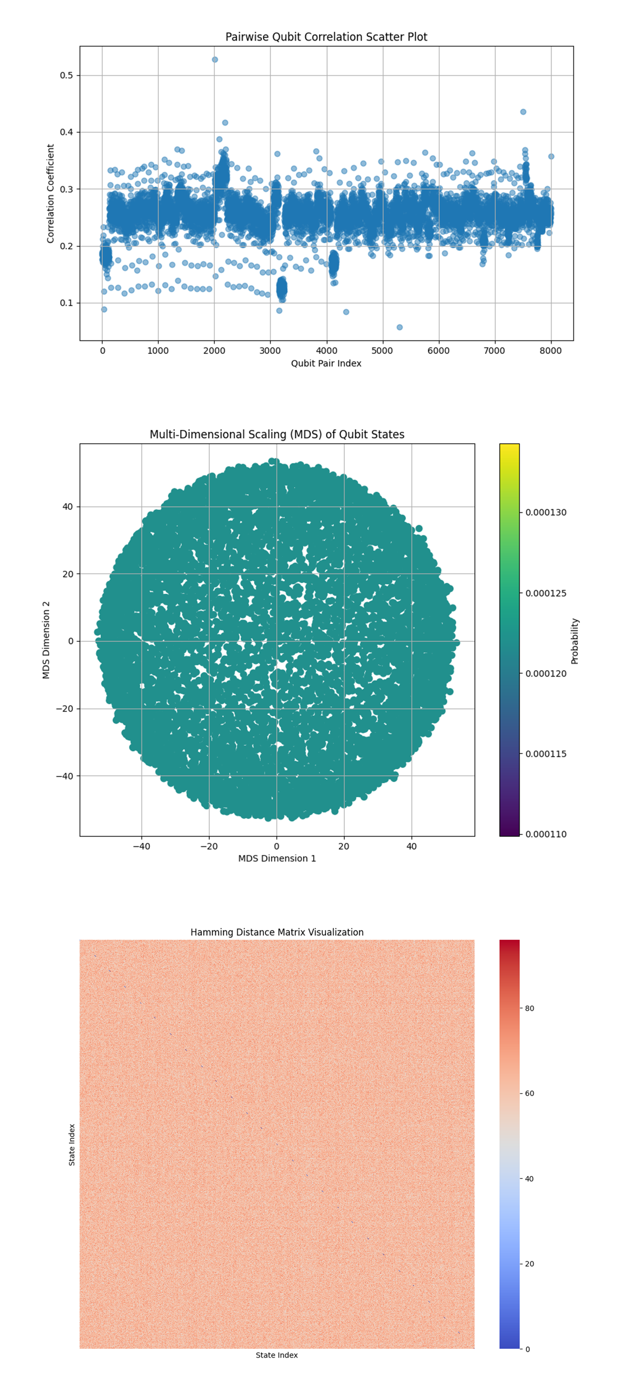
The scatter plot above (top) (code below) displays the correlation coefficients between pairs of qubits. The majority of correlations appear to be clustered between 0.2 and 0.3, with some outliers reaching up to 0.5.
For twistor theory, these correlations could represent how twistors, modeled as qubits, are interacting within the abstract quantum gravitational field. The strength of these correlations may reflect how abstract gravitational influences propagate through the network, affecting certain twistors more than others.
The range of correlation values suggests varying degrees of interaction across the network, indicating that the quantum gravitational effects are not uniformly distributed.
Higher correlation values between specific pairs indicates regions within the twistor network where abstract gravitational effects are stronger.
The presence of outliers might suggest areas of the network where twistors are more tightly linked, perhaps analogous to high-gravity regions in a quantum gravity model.
The MDS plot above (middle) (code below) shows the projection of high-dimensional qubit states into a 2D space, preserving the relative distances based on Hamming distances. The states appear to be uniformly spread within a circular pattern.
The circular pattern in the MDS plot might represent how twistor states are distributed within the high-dimensional twistor space under the influence of abstract quantum gravity. This uniform spread could suggest that the gravitational effects are distributed in a way that maintains some symmetry within the twistor network.
If we consider the circular spread as an analogy for the 'event horizon' of a gravitational system, this plot could be showing the boundary within which quantum gravitational effects are most pronounced. The uniformity might imply a certain level of coherence in how twistors interact, despite the perturbations.
The heatmap above (bottom) (code below) shows the Hamming distances between different measurement outcomes, with most distances appearing high (close to the maximum value for the system).
The high Hamming distances show that the outcomes are widely spread across the state space, with most states differing from each other by a large number of bit flips. This could indicate that the network has been influenced by a complex or highly dynamic abstract gravitational field.
The spread could also suggest that abstract quantum gravitational effects are strong, causing twistors to occupy a large variety of states with minimal coherence. This might align with theories where quantum gravity introduces significant fluctuations into the state space.
The large Hamming distances might correlate with the high entropy observed earlier, reinforcing the idea that the system is highly disordered. This is consistent with a scenario where quantum gravity destabilizes previously coherent structures within the twistor network.

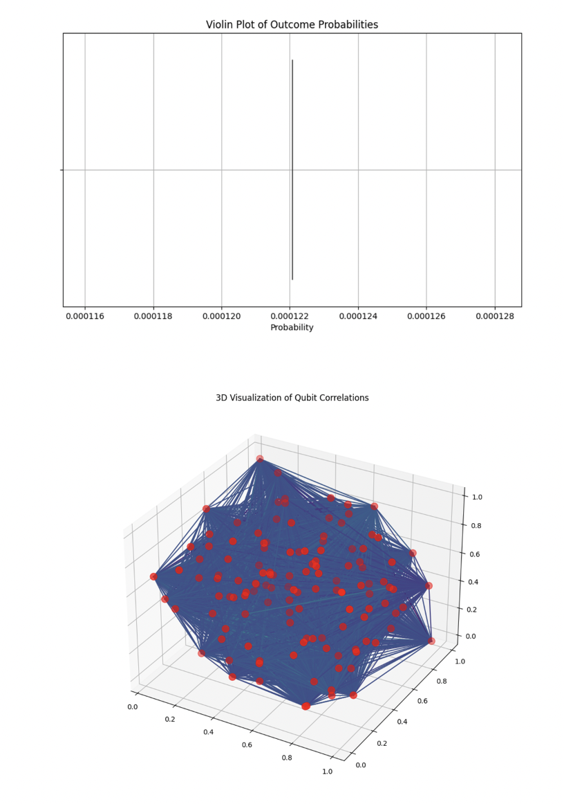
The violin plot above (top) (code below) shows a very narrow distribution of outcome probabilities, indicating that most outcomes have nearly identical probabilities.
The narrowness of the plot suggests that the quantum gravitational effects in the experiment have led to a situation where no specific outcomes are significantly more probable than others. This could imply that the gravitational influence is distributed in a way that flattens the probability landscape, leading to near-uniform outcome probabilities.
This uniformity might suggest that the quantum gravitational perturbations are causing a form of 'quantum thermalization', where the system explores a broad state space but with nearly equal likelihood for each state.
In twistor theory, this could indicate that the network of twistors is highly interconnected, with no single path or configuration dominating the probability space. This might reflect a scenario where quantum gravity prevents the formation of stable structures, leading to a uniform distribution across possible states.
The 3D scatter plot (top) (code below) shows qubits as points in space with edges representing correlations. The network of edges indicates that most qubits are connected through significant correlations.
The connectivity implies that the quantum gravitational effects have led to a highly entangled state, where most qubits are correlated with one another. This could represent a scenario where abstract gravitational effects cause widespread entanglement within the network. The 3D structure may suggest that these interactions are distributed across multiple dimensions of the twistor space.
In the end, the abstract quantum gravity experiment using twistor theory revealed a highly entangled, complex system with widespread correlations, a uniform distribution of state probabilities, and significant quantum entropy. The pairwise qubit correlation scatter plot highlighted varying degrees of interaction within the twistor network, while the MDS projection suggested a symmetrical distribution of states in the twistor space. The Hamming distance matrix emphasized the wide spread of outcomes, indicating strong abstract gravitational perturbations, and the violin plot confirmed a nearly uniform probability landscape.

Code:

# imports
import numpy as np
from qiskit import QuantumCircuit, ClassicalRegister, transpile
from qiskit_ibm_runtime import QiskitRuntimeService, Session, SamplerV2
from qiskit.visualization import plot_histogram  
import json
import matplotlib.pyplot as plt

# Initialize Qiskit Runtime Service
service = QiskitRuntimeService(
    channel='ibm_quantum',
    instance='ibm-q/open/main',
    token='YOUR_IBMQ_KEY_O-`'
)

# Define the backend
backend = service.backend('ibm_kyoto')

# Create a Quantum Circuit with 127 qubits 
num_qubits = 127
qc = QuantumCircuit(num_qubits)

# Classical register for measurement
classical_reg = ClassicalRegister(num_qubits)
qc.add_register(classical_reg)

# Step 1: Initialize each twistor node in superposition
for qubit in range(num_qubits):
    qc.h(qubit)  # Hadamard gate to create superposition

# Step 2: Model twistor propagation by introducing entanglement
for qubit in range(0, num_qubits - 1, 2):
    qc. cz(qubit, qubit + 1)  # Controlled-Z gate for entanglement

# Step 3: Apply rotations to model quantum gravitational effects
for qubit in range(num_qubits):
    theta_x = np.random.uniform(0, 2 * np.pi)
    theta_y = np.random.uniform(0, 2 * np.pi)
    theta_z = np.random.uniform(0, 2 * np.pi)
    qc.rx(theta_x, qubit)
    qc.ry(theta_y, qubit)
    qc.rz(theta_z, qubit)

# Step 4: Add additional entanglement to model more complex interactions
for qubit in range(0, num_qubits - 2, 3):
    qc. cx(qubit, qubit + 2)  # Controlled-X gate for further entanglement

# Step 5: Measure all qubits
qc.measure(range(num_qubits), range(num_qubits))

# Transpile the circuit on ibm_kyoto 
transpiled_qc = transpile(qc, backend=backend, optimization_level=3)

# Execution on backend with SamplerV2
with Session(service=service, backend=backend) as session:
    sampler = SamplerV2(session=session)
    
    # Run the circuit 
    job = sampler. run([transpiled_qc], shots=8192)
    job_result = job.result()
    
    # Retrieve the classical register name
    classical_register = qc.cregs[0].name

    # Extract counts for the first (and only) pub result
    pub_result = job_result[0].data[classical_register].get_counts()

    # Save the results to JSON
    results_data = {
        "raw_counts": pub_result
    }
    
    file_path = '/Users/Documents/gravitational_instanton_results.json'
    with open(file_path, 'w') as f:
        json.dump(results_data, f, indent=4)

# Plotting the results 
plot_histogram(pub_result)
plt. show()

# End.

///////////////////////////////////////////////////////////////////

Histogram, Heatmap of Qubit Correlations, Entropy Analysis, and State Distribution Analysis (Hamming Weight) Visuals from Run Data.
# imports
import json
import numpy as np
from qiskit.visualization import plot_histogram
import matplotlib.pyplot as plt
import seaborn as sns
from scipy.stats import entropy

# Load results from JSON
file_path = '/Users/Documents/gravitational_instanton_results.json'
with open(file_path, 'r') as f:
    results_data = json.load(f)

# Extract raw counts from the results data
raw_counts = results_data["raw_counts"]

# Display the raw counts to understand the distribution
print("Raw counts from the experiment:")
print(raw_counts)

# Total number of qubits
num_qubits = len(next(iter(raw_counts.keys())))

# 1. Histogram of Measurement Outcomes
plt.figure(figsize=(12, 8))
plot_histogram(raw_counts)
plt.title("Histogram of Measurement Outcomes")
plt. show()

# 2. Heatmap of Qubit Correlations
# Create a correlation matrix from the raw counts
correlation_matrix = np.zeros((num_qubits, num_qubits))

for outcome, count in raw_counts.items():
    outcome_array = np.array([int(bit) for bit in outcome])
    for i in range(num_qubits):
        for j in range(num_qubits):
            if i != j:
                correlation_matrix[i, j] += outcome_array[i] * outcome_array[j] * count

# Normalize the correlation matrix
correlation_matrix /= sum(raw_counts.values())

# Plot the heatmap of the correlation matrix
plt.figure(figsize=(12, 10))
sns.heatmap(correlation_matrix, cmap='coolwarm', annot=False)
plt.title("Heatmap of Qubit Correlations")
plt. show()

# 3. Entropy Analysis
# Calculate the probability distribution from raw counts
total_shots = sum(raw_counts.values())
probability_distribution = np.array([count / total_shots for count in raw_counts.values()])

# Calculate entropy of the system
system_entropy = entropy(probability_distribution, base=2)

# Display entropy
print(f"System Entropy: {system_entropy:.4f} bits")

# Visualize the entropy on a bar chart
plt.figure(figsize=(8, 6))
plt. bar(["Entropy"], [system_entropy], color='teal')
plt.title("Entropy of the Twistor Network")
plt.ylabel("Entropy (bits)")
plt. show()

# 4. State Distribution Analysis (Hamming Weight)
# Calculate the Hamming weight for each outcome and count the occurrences
hamming_weights = {}
for outcome, count in raw_counts.items():
    weight = outcome.count('1')
    if weight in hamming_weights:
        hamming_weights[weight] += count
    else:
        hamming_weights[weight] = count

# Normalize the Hamming weight distribution
for weight in hamming_weights:
    hamming_weights[weight] /= total_shots

# Plot the distribution of Hamming weights
plt.figure(figsize=(10, 6))
plt. bar(hamming_weights.keys(), hamming_weights.values(), color='coral')
plt.title("Distribution of Hamming Weights")
plt.xlabel("Hamming Weight")
plt.ylabel("Probability")
plt. show()

# End.

////////////////////////////////////////////////////////////////

Bitstring Cluster Analysis, Distribution of Hamming Distances, and Fourier Transform of Bitstrings Visuals from Run Data
# imports
import json
import numpy as np
import matplotlib.pyplot as plt
from itertools import combinations

# Load the results from JSON
file_path = '/Users/Documents/qft_twistor_experiment_results.json'
with open(file_path, 'r') as file:
    results = json.load(file)

# Extract raw counts
counts = results['raw_counts']

# Convert bitstrings to a list of integers
bitstrings = list(counts.keys())
bitstring_frequencies = list(counts.values())

# Convert bitstrings to numpy array 
bit_array = np.array([[int(bit) for bit in bitstring] for bitstring in bitstrings])

# Visualization 1: Bitstring Cluster Analysis
from sklearn.decomposition import PCA
from sklearn.cluster import KMeans

# Apply PCA to reduce dimensionality
pca = PCA(n_components=2)
bitstring_pca = pca. fit_transform(bit_array)

# Apply KMeans clustering
kmeans = KMeans(n_clusters=5)
clusters = kmeans. fit_predict(bitstring_pca)

# Plot the PCA-transformed bitstrings 
plt.figure(figsize=(10, 6))
plt.scatter(bitstring_pca[:, 0], bitstring_pca[:, 1], c=clusters, cmap='viridis')
plt.title('Bitstring Cluster Analysis with PCA')
plt.xlabel('PCA Component 1')
plt.ylabel('PCA Component 2')
plt.colorbar(label='Cluster')
plt. show()

# Visualization 2: Distribution of Hamming Distances
def hamming_distance(s1, s2):
    """Calculate the Hamming distance between two bitstrings."""
    return sum(c1 != c2 for c1, c2 in zip(s1, s2))

# Calculate all pairwise Hamming distances
hamming_distances = [hamming_distance(b1, b2) for b1, b2 in combinations(bitstrings, 2)]

# Plot the distribution of Hamming distances
plt.figure(figsize=(10, 6))
plt.hist(hamming_distances, bins=range(128), color='purple', edgecolor='black')
plt.xlabel('Hamming Distance')
plt.ylabel('Frequency')
plt.title('Distribution of Hamming Distances Between Bitstrings')
plt. show()

# Visualization 3: Fourier Transform of Bitstrings
def bitstring_to_int(bitstring):
    """Convert a bitstring to an integer."""
    return int(bitstring, 2)

# Convert bitstrings to integers
bitstring_ints = [bitstring_to_int(bitstring) for bitstring in bitstrings]

# Apply Fourier transform
fft_result = np.fft.fft(bitstring_ints)
fft_magnitude = np.abs(fft_result)

# Plot the magnitude of the Fourier transform
plt.figure(figsize=(10, 6))
plt.plot(fft_magnitude, color='orange')
plt.xlabel('Frequency Component')
plt.ylabel('Magnitude')
plt.title('Fourier Transform of Bitstrings')
plt. show()

# End.