Conformal Invariance in Quantum Field Theory (127-Qubits)

This experiment explores the application of twistor theory and conformal invariance within the framework of quantum field theory (QFT). Using IBM's 127-qubit quantum computer (ibm_brisbane) and qiskit, this experiment implements a quantum circuit that simulates field interactions governed by conformal symmetries. The circuit is structured to encode twistor states, apply complex conformal transformations (including rotations, dilations, and translations), and measure the outcomes to analyze potential emergent symmetries.

1. Initialization and Setup
We define a quantum circuit (qc) with 127 qubits and 127 classical bits.
qc = QuantumCircuit(127, 127)
Calibration data for the backend (ibm_brisbane) is loaded from a CSV file. This data includes errors for various quantum gates such as RZ, SX, and ECR, as well as readout errors.
calibration_data = pd. read_csv(calibration_data_path)
The mean values of these errors are computed to understand the performance characteristics of the backend.
avg_rz_error = calibration_data[′Z-axis rotation (rz) error ′].mean()
avg_sx_error = calibration_data[′√x (sx) error ′].mean()
avg_ecr_error = calibration_data[′ECR error ′].mean()
avg_readout_error = calibration_data[′Readout assignment error ′].mean()

2. Twistor State Initialization
Each qubit in the circuit is initialized into a superposition state using the Hadamard gate.
qc.h(i)
Subsequent rotations are applied to encode the twistor state. These rotations use the following gates:
RZ Gate: Rotates the qubit around the Z-axis by an angle of π/4​.
qc.rz(4/π​, i)
RX Gate: Rotates the qubit around the X-axis by an angle of π/3​.
qc.rx(π/3, i)
RY Gate: Rotates the qubit around the Y-axis by an angle of π/6​.
qc.ry(π/6, i)

3. Application of Complex Conformal Transformations
We apply conformal rotations using a combination of controlled-RZ (CRZ), controlled-RX (CRX), and controlled-RY (CRY) gates. These transformations simulate the rotational symmetries in twistor space.
CRZ Gate: Applies a controlled rotation around the Z-axis by π/4​.
qc.crz(4/π​, i, i + 2)
CRX Gate: Applies a controlled rotation around the X-axis by π/3​.
qc.crx(3/π​, i + 1, i + 3)
CRY Gate: Applies a controlled rotation around the Y-axis by π/6.
qc.cry(6/π​, i + 2, i + 4)
A custom unitary gate, representing a specific conformal transformation in twistor space, is created and applied. This gate is based on a 4x4 matrix constructed from the Kronecker product of a 2x2 rotation matrix and the identity matrix.
custom_unitary = np.kron(small_unitary, np.eye(2))
The unitary gate is then applied across the qubits, controlled by adjacent qubits.
qc.append(unitary_gate.control(1), [i, i + 1, i + 2])
Conformal dilations are implemented using controlled-RX (CRX) and controlled-X (CX) gates. These transformations represent scaling symmetries.
CRX Gate: Applies a controlled rotation around the X-axis by π/2​.
qc.crx(2/π​, i, i + 5)
CX Gate: Applies a controlled-X gate (CNOT).
qc. cx(i + 1, i + 6)
Additional conformal transformations are applied using a deeper combination of controlled-RZ, controlled-RX, controlled-RY, and controlled-X gates.
qc.crz(8/π​, i, i + 6)
qc.crx(7/π​, i + 1, i + 7)
qc.cry(5/π​, i + 2, i + 8)
qc. cx(i + 3, i + 9)
qc.crz(6/π​, i + 4, i + 10)

4. Measurement in the Twistor Basis
Before measurement, each qubit is rotated back using the RX gate with an angle of −π/3.
qc.rx(−3/π​, i)
All qubits are then measured, and the results are stored in classical registers.
qc.measure(i, i)

5. Transpilation and Execution
The quantum circuit is transpiled to match the specific properties and calibration data of ibm_brisbane backend. The optimization level is set to 3.
transpiled_qc = transpile(qc, backend = backend, optimization_level = 3)
The circuit is executed on ibm_brisbane backend using SamplerV2. The number of shots is set to 8192.
job = sampler. run([transpiled_qc], shots = 8192)
The name of the classical register is retrieved, and the counts for the measurement outcomes are extracted.
classical_register = qc.cregs[0].name
pub_result = job_result[0].data[classical_register].get_counts()

6. Analysis and Visualization
The raw counts from the quantum computation are saved to a JSON.
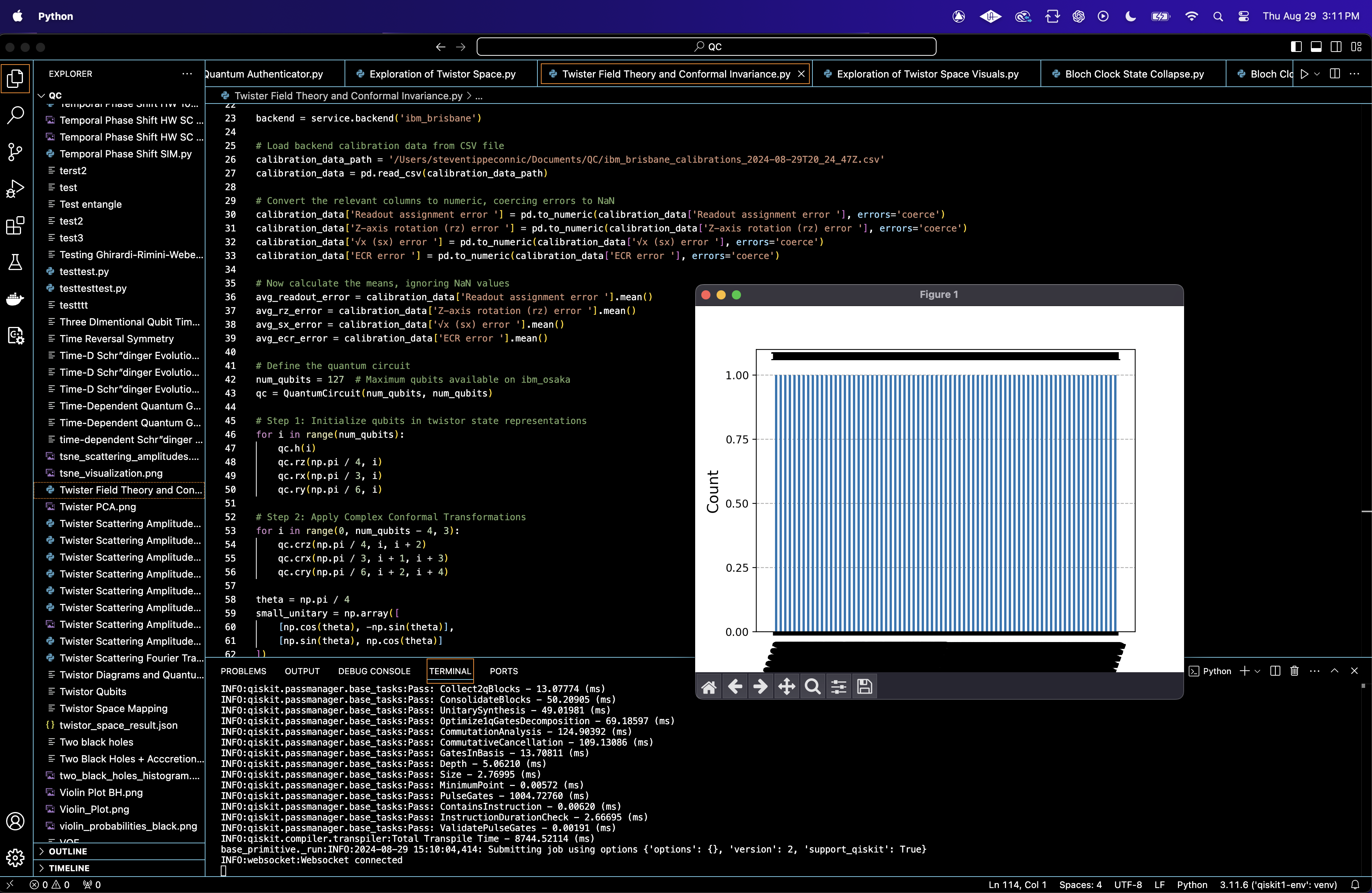
A histogram of the measurement outcomes is plotted to visually inspect the distribution and potential symmetries.

Results:
Shannon Entropy from run(code below) = 13.0000
A Shannon entropy of 13 is high, indicating that the quantum state after evolution is highly mixed and there is significant uncertainty in predicting any particular outcome.
In the context of exploring twistor space, this high entropy suggests that the state evolution led to a situation where all possible configurations are nearly equally probable, which is indicative of a highly complex, chaotic quantum system with deep entanglement and no simple, dominant structures.

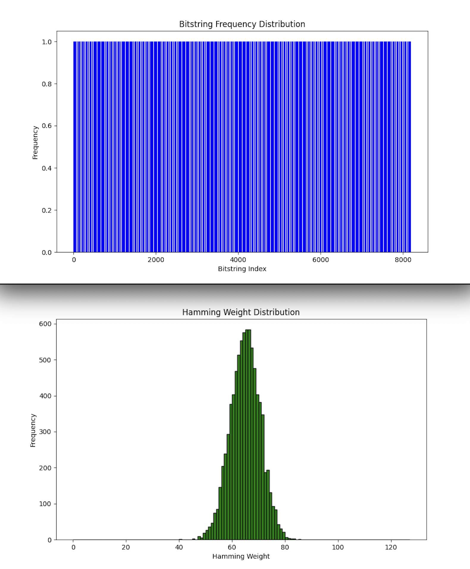
The Bitstring Frequency Distribution chart above (top) (code below) shows a nearly uniform distribution, with most bitstrings appearing with roughly the same frequency across the 8192 shots. This lack of dominant bitstrings suggests that the quantum circuit's configuration resulted in a highly entangled state space where no single configuration was more likely than others.
The uniform distribution may indicate that the quantum circuit effectively encoded conformal symmetry, as conformal invariance often implies that no specific configuration (bitstring) should be favored over others in the absence of explicit symmetry breaking.
The Hamming Weight Distribution above (bottom) (code below) is bell-shaped, with most bitstrings having a Hamming weight centered around 63-67. The distribution resembles a normal distribution, indicating a symmetric spread of 1s across the qubits.
The Hamming weight distribution's bell shape suggests that the circuit's operations led to a balanced and symmetric state configuration. This symmetry aligns with the idea of conformal invariance, where transformations (such as scaling and rotations) preserve the overall distribution of qubits in the quantum state. A normal distribution of Hamming weights implies that the circuit maintained a consistent degree of qubit excitation (number of 1s) across different bitstrings, which is consistent with the preservation of scale symmetry in conformal field theory.

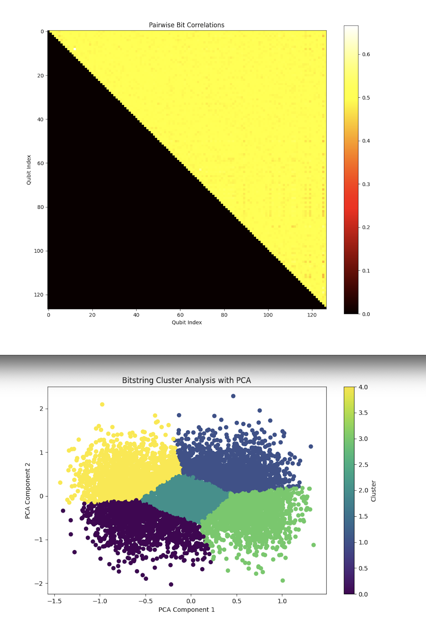
The Pairwise Bit Correlations heatmap above (top) (code below) reveals relatively high correlations (yellow regions) between many pairs of qubits, with a significant number of qubits showing similar measurement outcomes. The most correlated pairs appear towards the upper left and along the diagonal.
The strong correlations between certain qubits suggest that the quantum circuit induced some degree of coherence or collective behavior among these qubits. In the context of conformal field theory, these correlations may reflect the invariance under certain group transformations, where subsets of qubits transform similarly. This could be interpreted as a manifestation of local or global symmetries related to the conformal group. The presence of strong correlations might also indicate that certain conformal transformations (like rotations or dilations) were more dominant in the run.
The PCA (Principal Component Analysis) above (bottom) (code below) applied to the bitstrings and visualized in the cluster analysis shows distinct clusters in the reduced 2D space. Each cluster represents a group of bitstrings that share similar properties.
The formation of distinct clusters suggests that the quantum circuit generated bitstrings that naturally grouped into specific configurations. These clusters could correspond to different symmetry sectors of the conformal field theory, where each cluster represents a class of states invariant under certain conformal transformations.
The presence of clusters might also indicate that the twistor-based representation led to stable configurations in the quantum field, which could be a direct consequence of the circuit's encoding of conformal symmetries. These clusters can be interpreted as different 'phases' or 'sectors' of the quantum field, each preserving symmetries.

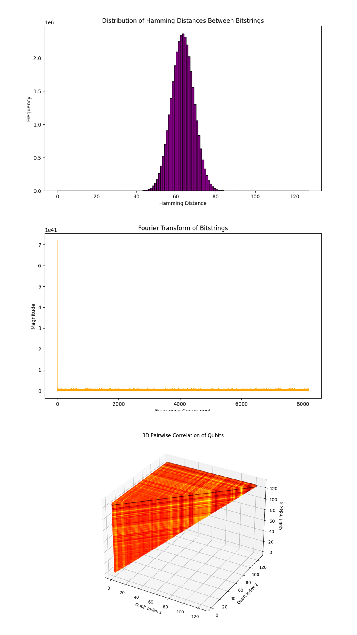
The distribution of Hamming distances between pairs of bitstrings above (top) (code below) shows a bell-shaped curve, centered around a specific Hamming distance (roughly between 60 and 70). The bell-shaped distribution suggests that most bitstrings are at a similar Hamming distance from each other, indicating a uniform spread of differences across the bitstrings. This uniformity could be interpreted as a sign of conformal symmetry preservation, where local interactions between qubits (encoded by the circuit) maintain a consistent degree of difference between quantum states.
In QFT, this distribution could correspond to the spread of field configurations in the Hamming space, where the quantum circuit ensures that field states remain close to each other in terms of qubit activations, preserving the local structure imposed by conformal symmetry.
The Fourier transform of the bitstrings above (middle) (code below) reveals a significant peak at the zero frequency component, with a relatively flat distribution of the other frequency components.
The prominent peak at zero frequency suggests that there is a dominant DC component, meaning that on average, the bitstrings are relatively uniform in their configuration. The flat distribution of other frequency components indicates a lack of periodic structure in the bitstrings, which could imply that the circuit did not induce any strong periodic patterns or oscillations in the state space.
The absence of significant higher-frequency components might suggest that the conformal transformations encoded by the circuit do not introduce periodic variations in the field configurations. This could be consistent with a field theory where scale invariance (a key aspect of conformal invariance) suppresses the formation of periodic structures, leading to a more homogeneous state space.
The 3D pairwise correlation visualization above (bottom) (code below) shows a dense grid-like structure with noticeable patterns of correlations across different qubit triplets. The intensity of the correlations is represented by the color scale, with brighter regions indicating stronger correlations.
The grid-like patterns and strong correlations between certain qubit triplets suggest that the quantum circuit has encoded non-trivial interactions between groups of three qubits, potentially reflecting higher-order symmetries in the simulated field theory. These triplet interactions could be indicative of complex conformal transformations that involve multiple qubits simultaneously, rather than simple pairwise interactions.
The consistent and strong correlations across the grid imply that certain configurations of qubits are favored, likely due to the preservation of symmetries within the quantum field. These invariant configurations could correspond to fixed points or attractors in the field theory, where the field remains stable under conformal transformations.
The visualization suggests that the quantum circuit may have created significant multi-qubit entanglement, where groups of qubits are correlated in such a way that they exhibit collective behavior. This entanglement is crucial for representing the complex interactions and symmetries inherent in conformal field theories, particularly those described by twistor theory.
In the end, the bitstring and Hamming weight distributions, coupled with the pairwise and triplet qubit correlations, indicated that the circuit maintained uniformity and symmetry across the quantum states, reflecting the underlying conformal invariance. The 3D PCA and correlation visualizations further highlighted the presence of distinct symmetry sectors and intricate multi-qubit entanglements, suggesting that the circuit captured higher-dimensional symmetry structures consistent with twistor theory.

Code:

# imports
import numpy as np
from qiskit import QuantumCircuit, transpile
from qiskit_ibm_runtime import QiskitRuntimeService, Session, SamplerV2
from qiskit.circuit.library import UnitaryGate, RZGate, RXGate, RYGate, CXGate, CRXGate, CRYGate, CRZGate
from qiskit.quantum_info import Statevector
from qiskit.visualization import plot_histogram
import json
import logging
import matplotlib.pyplot as plt
import pandas as pd

# Logging
logging.basicConfig(level=logging. INFO)
logger = logging.getLogger(__name__)

# Load IBM Quantum account
service = QiskitRuntimeService(
    channel='ibm_quantum',
    instance='ibm-q/open/main',
    token='YOUR_IBMQ_KEY_O-`'  
)

backend = service.backend('ibm_brisbane')

# Load backend calibration data from CSV file
calibration_data_path = '/Users/Documents/ibm_brisbane_calibrations_2024-08-29T20_24_47Z.csv'
calibration_data = pd. read_csv(calibration_data_path)

# Convert the relevant columns to numeric, coercing errors to NaN
calibration_data['Readout assignment error '] = pd. to_numeric(calibration_data['Readout assignment error '], errors='coerce')
calibration_data['Z-axis rotation (rz) error '] = pd. to_numeric(calibration_data['Z-axis rotation (rz) error '], errors='coerce')
calibration_data['√x (sx) error '] = pd. to_numeric(calibration_data['√x (sx) error '], errors='coerce')
calibration_data['ECR error '] = pd. to_numeric(calibration_data['ECR error '], errors='coerce')

# Calculate the means
avg_readout_error = calibration_data['Readout assignment error '].mean()
avg_rz_error = calibration_data['Z-axis rotation (rz) error '].mean()
avg_sx_error = calibration_data['√x (sx) error '].mean()
avg_ecr_error = calibration_data['ECR error '].mean()

# Define the quantum circuit
num_qubits = 127  # Maximum qubits available on ibm_osaka
qc = QuantumCircuit(num_qubits, num_qubits)

# Step 1: Initialize qubits in twistor state representations
for i in range(num_qubits):
    qc.h(i)
    qc.rz(np.pi / 4, i)
    qc.rx(np.pi / 3, i)
    qc.ry(np.pi / 6, i)

# Step 2: Apply Complex Conformal Transformations
for i in range(0, num_qubits - 4, 3):
    qc.crz(np.pi / 4, i, i + 2)
    qc.crx(np.pi / 3, i + 1, i + 3)
    qc.cry(np.pi / 6, i + 2, i + 4)

theta = np.pi / 4
small_unitary = np.array([
    [np.cos(theta), -np.sin(theta)],
    [np.sin(theta), np.cos(theta)]
])
custom_unitary = np.kron(small_unitary, np.eye(2))
unitary_gate = UnitaryGate(custom_unitary)

for i in range(0, num_qubits - 3, 4):
    qc.append(unitary_gate.control(1), [i, i + 1, i + 2])

for i in range(0, num_qubits - 6, 5):
    qc.crx(np.pi / 2, i, i + 5)
    qc. cx(i + 1, i + 6)

for i in range(0, num_qubits - 10, 6):
    qc.crz(np.pi / 8, i, i + 6)
    qc.crx(np.pi / 7, i + 1, i + 7)
    qc.cry(np.pi / 5, i + 2, i + 8)
    qc. cx(i + 3, i + 9)
    qc.crz(np.pi / 6, i + 4, i + 10)

# Step 3: Measure in the twistor basis
for i in range(num_qubits):
    qc.rx(-np.pi / 3, i)
    qc.measure(i, i)

# Transpile the circuit 
transpiled_qc = transpile(qc, backend=backend, optimization_level=3)

# Execution with SamplerV2
with Session(service=service, backend=backend) as session:
    sampler = SamplerV2(session=session)
    
    # Run the circuit 
    job = sampler. run([transpiled_qc], shots=8192)
    job_result = job.result()
    
    # Retrieve the classical register name
    classical_register = qc.cregs[0].name

    # Extract counts for the first (and only) pub result
    pub_result = job_result[0].data[classical_register].get_counts()

    # Save the results to JSON
    results_data = {
        "raw_counts": pub_result
    }
    
    file_path = '/Users/Documents/qft_twistor_experiment_results.json'
    with open(file_path, 'w') as f:
        json.dump(results_data, f, indent=4)

# Plotting the results 
plot_histogram(pub_result)
plt. show()

# End

///////////////////////////////////////////////////////////////////

Code for Bitstring Frequency Distribution Visual, Hamming Weight Distribution Visual, and Pairwise Bit Correlations Visual from Run Data
# imports
import json
import matplotlib.pyplot as plt
from collections import Counter
import numpy as np

# Load the results from JSON
file_path = '/Users/Documents/qft_twistor_experiment_results.json'
with open(file_path, 'r') as file:
    results = json.load(file)

# Extract raw counts
counts = results['raw_counts']

# Plot 1: Bitstring Frequency Distribution
bitstring_frequencies = Counter(counts)
plt.figure(figsize=(10, 6))
plt. bar(range(len(bitstring_frequencies)), list(bitstring_frequencies.values()), color='blue')
plt.xlabel('Bitstring Index')
plt.ylabel('Frequency')
plt.title('Bitstring Frequency Distribution')
plt. show()

# Plot 2: Hamming Weight Distribution
hamming_weights = [bitstring.count('1') for bitstring in counts.keys()]
plt.figure(figsize=(10, 6))
plt.hist(hamming_weights, bins=range(128), color='green', edgecolor='black')
plt.xlabel('Hamming Weight')
plt.ylabel('Frequency')
plt.title('Hamming Weight Distribution')
plt. show()

# Plot 3: Pairwise Bit Correlations
num_qubits = 127
correlation_matrix = np.zeros((num_qubits, num_qubits))
for bitstring in counts.keys():
    for i in range(num_qubits):
        for j in range(i+1, num_qubits):
            if bitstring[i] == bitstring[j]:
                correlation_matrix[i, j] += 1
total_shots = sum(counts.values())
correlation_matrix /= total_shots
plt.figure(figsize=(12, 10))
plt.imshow(correlation_matrix, cmap='hot', interpolation='nearest')
plt.colorbar()
plt.xlabel('Qubit Index')
plt.ylabel('Qubit Index')
plt.title('Pairwise Bit Correlations')
plt. show()

///////////////////////////////////////////////////////////////////

Code for the Bistring Cluster Analysis with PCA Visual, Distribution of Hamming Distances Between Bitstrings Visual, and Fourier Transform of Bitstrings Visual from Run Data
# imports
import json
import numpy as np
import matplotlib.pyplot as plt
from itertools import combinations

# Load the results from  JSON
file_path = '/Users/Documents/qft_twistor_experiment_results.json'
with open(file_path, 'r') as file:
    results = json.load(file)

# Extract raw counts
counts = results['raw_counts']

# Convert bitstrings to a list of integers
bitstrings = list(counts.keys())
bitstring_frequencies = list(counts.values())

# Convert bitstrings to numpy array
bit_array = np.array([[int(bit) for bit in bitstring] for bitstring in bitstrings])

# Visualization 1: Bitstring Cluster Analysis
from sklearn.decomposition import PCA
from sklearn.cluster import KMeans

# Apply PCA to reduce dimensionality
pca = PCA(n_components=2)
bitstring_pca = pca. fit_transform(bit_array)

# Apply KMeans clustering
kmeans = KMeans(n_clusters=5)
clusters = kmeans. fit_predict(bitstring_pca)

# Plot the PCA-transformed bitstrings with cluster coloring
plt.figure(figsize=(10, 6))
plt.scatter(bitstring_pca[:, 0], bitstring_pca[:, 1], c=clusters, cmap='viridis')
plt.title('Bitstring Cluster Analysis with PCA')
plt.xlabel('PCA Component 1')
plt.ylabel('PCA Component 2')
plt.colorbar(label='Cluster')
plt. show()

# Visualization 2: Distribution of Hamming Distances
def hamming_distance(s1, s2):
    """Calculate the Hamming distance between two bitstrings."""
    return sum(c1 != c2 for c1, c2 in zip(s1, s2))

# Calculate all pairwise Hamming distances
hamming_distances = [hamming_distance(b1, b2) for b1, b2 in combinations(bitstrings, 2)]

# Plot the distribution of Hamming distances
plt.figure(figsize=(10, 6))
plt.hist(hamming_distances, bins=range(128), color='purple', edgecolor='black')
plt.xlabel('Hamming Distance')
plt.ylabel('Frequency')
plt.title('Distribution of Hamming Distances Between Bitstrings')
plt. show()

# Visualization 3: Fourier Transform of Bitstrings
def bitstring_to_int(bitstring):
    """Convert a bitstring to an integer."""
    return int(bitstring, 2)

# Convert bitstrings to integers
bitstring_ints = [bitstring_to_int(bitstring) for bitstring in bitstrings]

# Apply Fourier transform
fft_result = np.fft.fft(bitstring_ints)
fft_magnitude = np.abs(fft_result)

# Plot the magnitude of the Fourier transform
plt.figure(figsize=(10, 6))
plt.plot(fft_magnitude, color='orange')
plt.xlabel('Frequency Component')
plt.ylabel('Magnitude')
plt.title('Fourier Transform of Bitstrings')
plt. show()

# End.

/////////////////////////////////////////////////////////////

Code for 3D Pairwise Correlation of Qubits Visual from Run Data
# imports
import json
import numpy as np
import matplotlib.pyplot as plt
from mpl_toolkits.mplot3d import Axes3D

# Load the results from JSON
file_path = '/Users/Documents/qft_twistor_experiment_results.json'
with open(file_path, 'r') as file:
    results = json.load(file)

# Extract raw counts
counts = results['raw_counts']

# Convert bitstrings to a list of integers
bitstrings = list(counts.keys())

# Convert bitstrings to numpy array 
bit_array = np.array([[int(bit) for bit in bitstring] for bitstring in bitstrings])

# Calculate pairwise correlations in 3D space
num_qubits = bit_array.shape[1]
correlation_matrix_3d = np.zeros((num_qubits, num_qubits, num_qubits))

# Calculate correlations for all triplet combinations of qubits
for i in range(num_qubits):
    for j in range(i+1, num_qubits):
        for k in range(j+1, num_qubits):
            correlation_matrix_3d[i, j, k] = np.mean(bit_array[:, i] * bit_array[:, j] * bit_array[:, k])

# Plot the 3D correlation matrix
fig = plt.figure(figsize=(12, 8))
ax = fig.add_subplot(111, projection='3d')

# Use non-zero correlations for plotting
non_zero_indices = np.nonzero(correlation_matrix_3d)
ax.scatter(non_zero_indices[0], non_zero_indices[1], non_zero_indices[2], c=correlation_matrix_3d[non_zero_indices], cmap='hot', depthshade=True)

ax.set_xlabel('Qubit Index 1')
ax.set_ylabel('Qubit Index 2')
ax.set_zlabel('Qubit Index 3')
ax.set_title('3D Pairwise Correlation of Qubits')

plt. show()

# End.