Quantum Exploration of Twistor Space (127-Qubits)
1. Initialization and Setup
We define a quantum circuit with 127 qubits, representing our system's degrees of freedom. Each qubit corresponds to a degree of freedom in the quantum state, which will be mapped to twistor space.
Initialize the quantum backend service using QiskitRuntimeService to establish communication with IBM’s ibm_kyoto.
2. Quantum State Preparation
The initial quantum state preparation is performed by applying random unitary operations to groups of qubits.
The qubits are grouped in sets of 2. For each group of qubits, a random unitary matrix U ∈ SU(2^k) is generated, where k is the group size.
3. Twistor Mapping
To simulate the mapping between space-time and twistor space, we apply controlled rotation gates:
A controlled rotation around the Y-axis is applied using the gate CRY(θ), where θ = π/6.
CRY(θ) =
(1, 0, 0, 0)
(0, cos(θ/2), 0 , -sin(θ/2))
(1, 0, 1, 0)
(0, sin(θ/2), 0, cos(θ/2))
A controlled rotation around the Z-axis is applied using the gate CRZ(θ) with the same angle θ = π/6.
CRZ(θ) =
(1, 0, 0, 0)
(0, e^(-iθ/2), 0, 0)
(0, 0, 1, 0)
(0, 0, 0, e^(iθ/2))
4. Twistor Operators
Additional unitary operations are applied to simulate twistor transformations. The same group-size approach is used to apply these operations:
Each unitary gate U is generated randomly within SU(2^k) for groups of qubits, where k is the number of qubits in the group.
The transformation equation remains:
∣ψ′⟩ = U∣ψ⟩
These operations are intended to mimic the complex mappings in twistor space.
5. Evolution of Quantum State
The quantum state is evolved through multiple rounds of random unitary transformations, reflecting dynamic changes in twistor space:
For each round, the quantum state is updated as:
∣ψ(n + 1)⟩ = U^(n)∣ψ^(n)⟩
where n indexes the rounds of evolution.
6. Measurement
After applying all unitary transformations and mappings, the quantum circuit is measured. The measurement collapses the quantum state into a classical bit string representing the outcome of the experiment:
Outcome = ∣x⟩ with probability ∣⟨x∣ψ⟩∣^2
The measurement is performed across all 127 qubits, resulting in a binary string representing the final quantum state.
7. Transpilation
The circuit is transpiled with optimization level 3 to ensure it is compatible with the backend's hardware constraints and to reduce the gate count where possible.
8. Execution on Backend
The circuit is executed on ibm_kyoto using SamplerV2. The shots parameter is set to 8192, meaning the circuit is repeated 8192 times to obtain a statistical distribution of results.
9. Post-Processing and Visualization
The result is extracted using the job’s result object, specifically targeting the counts from the classical register.
Counts = GetCounts(classical_register)
The counts are saved to a JSON.
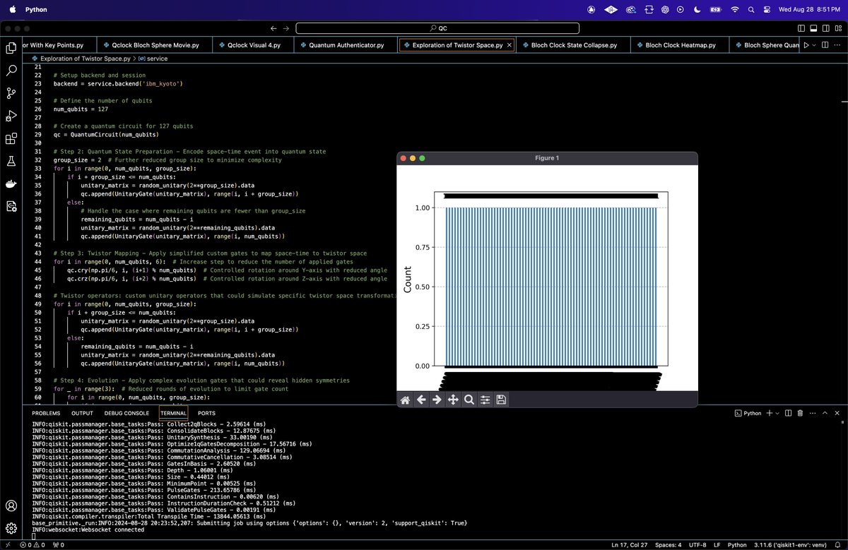
A histogram of the measurement results is plotted to visualize the distribution of the final quantum state across the possible outcomes.
Shannon Entropy from run(code below) = 13.0000
A Shannon entropy of 13 is high, indicating that the quantum state after evolution is highly mixed and there is significant uncertainty in predicting any particular outcome.
In the context of exploring twistor space, this high entropy suggests that the state evolution led to a situation where all possible configurations are nearly equally probable, which is indicative of a highly complex, chaotic quantum system with deep entanglement and no simple, dominant structures.

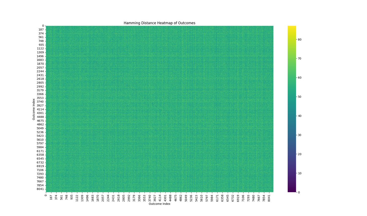
The Hamming Distance Heatmap above (code below) is a visualization of the pairwise Hamming distances between all observed outcomes for the run.
The heatmap shows a nearly uniform distribution, with the color intensity spread evenly across the matrix. This suggests that there is no strong clustering of similar outcomes; instead, the outcomes are quite evenly distributed in terms of their Hamming distances. This uniformity indicates a high level of entanglement and complexity in the quantum state, as expected from a run that involves complex mappings to twistor space.

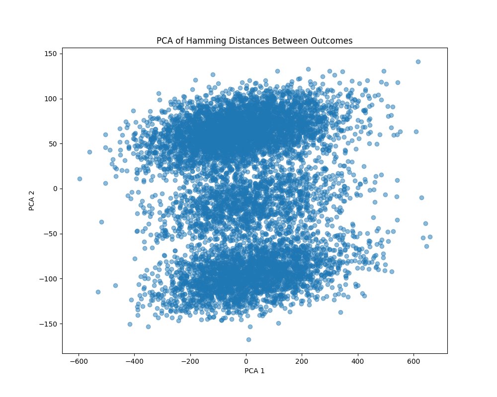
The PCA plot above (code below) reveals a two-layered structure with dense regions at the top and bottom and sparser regions in between. This structure suggests that while the quantum states differ significantly (as indicated by the Hamming distances), there are still underlying symmetries or patterns that group certain outcomes together.
In the context of twistor space, this layered structure could correspond to different 'slices' or sections of the twistor space where certain geometric properties dominate. It suggests that, although the state is highly complex, there are still coherent structures within the quantum state that reflect some aspects of the twistor mappings.

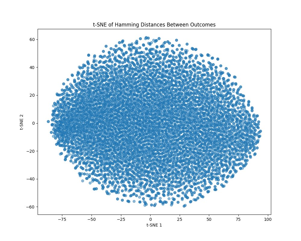
The t-SNE plot above (code below) shows a uniform, almost circular spread of the data points. Unlike PCA, t-SNE is nonlinear and is better at preserving local similarities, which suggests that despite the global complexity, locally, the outcomes are still quite uniformly distributed. This circular distribution may indicate that while the outcomes are uniformly spread, the underlying quantum state has a continuous symmetry, possibly reflecting the complex rotational symmetries of twistor space. This uniform spread also supports the idea that the quantum state is highly entangled and mixed, with no simple or isolated geometric features dominating the distribution. Analysis
The Hamming Distance Heatmap and the t-SNE analysis suggest that the quantum state, after evolution through the twistor mapping, is uniformly complex. This supports the idea that the mappings effectively captured the high-dimensional and intricate nature of twistor space.
The PCA analysis revealed some underlying structure, indicating that despite the overall complexity, there might be certain complex symmetries or geometric features of twistor space that are preserved in the quantum state.
The high Shannon entropy confirms that the quantum state is highly mixed, with no particular outcome being significantly more probable than others. This is consistent with the hypothesis that the evolution led to a state that thoroughly explored the available Hilbert space, reflecting the complexity of twistor space.
In the end, the experiment effectively captured the complex and high-dimensional nature of twistor space, by the uniform distribution of Hamming distances, the high entropy, and the layered structure revealed by PCA. The results suggest that the quantum state’s evolution led to an exploration of the twistor space, with significant entanglement and a complex distribution of outcomes. This aligns with the theoretical expectations of how a quantum system should behave when simulating twistor mappings, showing the potential of quantum computing for exploring higher-dimensional geometric spaces.
Code:
# imports
import numpy as np
from qiskit import QuantumCircuit, transpile
from qiskit_ibm_runtime import QiskitRuntimeService, Session, SamplerV2
from qiskit.quantum_info import random_unitary
from qiskit.circuit.library import UnitaryGate
from qiskit.visualization import plot_histogram
import json
import logging
import matplotlib.pyplot as plt

# Logging setup
logging.basicConfig(level=logging. INFO)
logger = logging.getLogger(__name__)

# Step 1: Load IBMQ
service = QiskitRuntimeService(
    channel='ibm_quantum',
    instance='ibm-q/open/main',
    token='YOUR_IBMQ_KEY_O-`'
)

# Setup backend and session
backend = service.backend('ibm_kyoto')

# Define number of qubits
num_qubits = 127

# Create a quantum circuit for 127 qubits
qc = QuantumCircuit(num_qubits)

# Step 2: Quantum State Preparation - Encode space-time event into quantum state
group_size = 2
for i in range(0, num_qubits, group_size):
    if i + group_size <= num_qubits:
        unitary_matrix = random_unitary(2**group_size).data
        qc.append(UnitaryGate(unitary_matrix), range(i, i + group_size))
    else:
        # Handle a case where remaining qubits are fewer than group_size
        remaining_qubits = num_qubits - i
        unitary_matrix = random_unitary(2**remaining_qubits).data
        qc.append(UnitaryGate(unitary_matrix), range(i, num_qubits))

# Step 3: Twistor Mapping - Apply simplified custom gates to map space-time to twistor space
for i in range(0, num_qubits, 6):  # Increase step to reduce the number of applied gates
    qc.cry(np.pi/6, i, (i+1) % num_qubits)  # Controlled rotation around Y-axis
    qc.crz(np.pi/6, i, (i+2) % num_qubits)  # Controlled rotation around Z-axis
# Twistor operators: custom unitary operators that could simulate specific twistor space transformations
for i in range(0, num_qubits, group_size):
    if i + group_size <= num_qubits:
        unitary_matrix = random_unitary(2**group_size).data
        qc.append(UnitaryGate(unitary_matrix), range(i, i + group_size))
    else:
        remaining_qubits = num_qubits - i
        unitary_matrix = random_unitary(2**remaining_qubits).data
        qc.append(UnitaryGate(unitary_matrix), range(i, num_qubits))

# Step 4: Evolution - Apply complex evolution gates for _ in range(3):
    for i in range(0, num_qubits, group_size):
        if i + group_size <= num_qubits:
            unitary_matrix = random_unitary(2**group_size).data
            qc.append(UnitaryGate(unitary_matrix), range(i, i + group_size))
        else:
            remaining_qubits = num_qubits - i
            unitary_matrix = random_unitary(2**remaining_qubits).data
            qc.append(UnitaryGate(unitary_matrix), range(i, num_qubits))

# Step 5: Measurement
qc.measure_all()

# Step 6: Transpilation backend and calibration data
transpiled_qc = transpile(qc, backend=backend, optimization_level=3)

# Execution on backend with SamplerV2
with Session(service=service, backend=backend) as session:
    sampler = SamplerV2(session=session)

    # Run the circuit
    job = sampler. run([transpiled_qc], shots=8192)
    job_result = job.result()

    # Retrieve the classical register name
    classical_register = qc.cregs[0].name

    # Extract counts for the first (and only) pub result
    pub_result = job_result[0].data[classical_register].get_counts()

    # Save the results to JSON
    results_data = {
        "raw_counts": pub_result
    }

    file_path = '/Users/Documents/twistor_space_result.json'
    with open(file_path, 'w') as f:
        json.dump(results_data, f, indent=4)

# Plotting the results for analysis
plot_histogram(pub_result)
plt. show()

logger. info("Twistor space exploration experiment completed successfully.")

# end

////////////////////////////////////////////////////////////////////

Code for Hamming Distance Calculation, Hamming Distance Heatmap Visual, Entropy Calculation, PCA Visualization, and t-SNE Visualization from Run Data
# imports
import json
import numpy as np
import matplotlib.pyplot as plt
import seaborn as sns
from collections import Counter
from scipy.spatial.distance import pdist, squareform
from sklearn.decomposition import PCA
from sklearn.manifold import TSNE

# Load the results from IBMQ Run
file_path = '/Users/Documents/twistor_space_result.json'
with open(file_path, 'r') as file:
    data = json.load(file)

# Extract the binary outcomes
outcomes = list(data['raw_counts'].keys())
num_outcomes = len(outcomes)

# Convert binary strings to integers for easier handling
int_outcomes = [int(outcome, 2) for outcome in outcomes]

# Hamming Distance Calculation
hamming_distances = np.zeros((num_outcomes, num_outcomes))
for i in range(num_outcomes):
    for j in range(i+1, num_outcomes):
        hamming_distances[i, j] = sum(c1 != c2 for c1, c2 in zip(outcomes[i], outcomes[j]))
        hamming_distances[j, i] = hamming_distances[i, j]

# Hamming Distance Heatmap Visualization
plt.figure(figsize=(10, 8))
sns.heatmap(hamming_distances, cmap='viridis')
plt.title('Hamming Distance Heatmap of Outcomes')
plt.xlabel('Outcome Index')
plt.ylabel('Outcome Index')
plt. show()

# Entropy Calculation
counts = np.array(list(data['raw_counts'].values()))
probabilities = counts / sum(counts)
entropy = -np.sum(probabilities * np.log2(probabilities))
print(f"Shannon Entropy of Outcomes: {entropy:.4f}")

# PCA Visualization
pca = PCA(n_components=2)
pca_result = pca. fit_transform(hamming_distances)
plt.figure(figsize=(10, 8))
plt.scatter(pca_result[:, 0], pca_result[:, 1], alpha=0.5)
plt.title('PCA of Hamming Distances Between Outcomes')
plt.xlabel('PCA 1')
plt.ylabel('PCA 2')
plt. show()

# t-SNE Visualization
tsne = TSNE(n_components=2, perplexity=30.0)
tsne_result = tsne. fit_transform(hamming_distances)
plt.figure(figsize=(10, 8))
plt.scatter(tsne_result[:, 0], tsne_result[:, 1], alpha=0.5)
plt.title('t-SNE of Hamming Distances Between Outcomes')
plt.xlabel('t-SNE 1')
plt.ylabel('t-SNE 2')
plt. show()

# End.
