Quantum Computation of Scattering Amplitudes Using Twistor Theory on a 127-Qubit IBM Quantum Computer
1. Initialization of the Quantum Circuit
We initialize a quantum circuit with 127 qubits and 127 classical bits. The number of qubits represents the number of particles or degrees of freedom in the scattering process.
The classical bits are used to store the measurement results of each qubit.
Quantum Circuit: C(n, n) where n = 127
2. Random Initialization of Qubit States
Each qubit is initialized to represent a possible quantum state of a particle involved in the scattering process.
For each qubit q_i (where i = 0, 1, …, 126), we apply a rotation around the Y-axis using a randomly generated angle θ_i.
R_Y(θ_i) = exp(−i(θ_i/2)σ_y)
where θ_i is a random angle between 0 and 2π.
3. Entanglement to Simulate Particle Interactions
To simulate the interactions between particles, we entangle pairs of qubits.
We apply CNOT (Controlled-NOT) gates between adjacent qubits (q_i, q_(i+1)) for i = 0, 2, 4, …, 124.
CNOT(q_i, q_(i+1)) =
(I, 0)
(0, X)
where I is the identity matrix and X is the Pauli-X matrix (NOT gate).
4. Twistor-Inspired Unitary Transformations
Twistor theory provides a geometric framework that simplifies the computation of scattering amplitudes. This simulates this by applying unitary transformations to each qubit.
For each qubit q_i, we generate a random 2x2 unitary matrix U_i and apply it as a gate.
U_i = U(2) where U(2) is a unitary matrix satisfying U_(i)^† U_i = I
The matrix U_i is generated using the Haar measure to ensure it is unitary.
5. Additional Entanglement to Simulate Higher-Order Interactions
To simulate more complex interactions, this introduces additional entanglement between non-adjacent qubits.
We apply CNOT gates between qubits (q_i, q_(i+2)) and (q_(i + 1), q_(i + 3)) for i = 0, 4, 8, …, 120.
CNOT(q_i, q_(i+2)) and CNOT(q_(i + 1), q_(i+3))
6. Final Rotations to Encode Scattering Amplitudes
We apply a final set of rotations around the Z-axis to encode information about the scattering amplitudes.
For each qubit q_i, a rotation gate R_Z(ϕ_i) is applied with a randomly generated angle ϕ_i.
R_Z(ϕ_i) = exp(−i(ϕ_i/2)σ_z)
where ϕ_i is a random angle between 0 and 2π.
7. Measurement of Qubit States
The final state of each qubit is measured and stored in the corresponding classical bit. These measurements represent the outcome of the scattering process.
Each qubit q_i is measured, and the result is stored in the classical register c_i.
M(q_i) → c_i for i = 0, 1, …, 126
8. Transpilation and Optimization
The quantum circuit is transpiled for the IBM 127-qubit quantum computer ibm_brisbane. This performs optimization using Qiskit’s transpiler with an optimization level of 3, focusing on reducing gate depth and error rates.
9. Execution on the IBM Quantum Backend
The quantum circuit is executed on ibm_brisbane.
The circuit is run with 8192 shots.
Run(C, shots = 8192)
10. Extraction of Scattering Amplitudes
The measurement results (counts) are used to compute the scattering amplitudes, which represent the probabilities of different outcomes of the scattering process.
The counts are normalized to convert them into probabilities (scattering amplitudes).
P_i = counts(c_i)/total counts
11. Saving and Visualization of Results
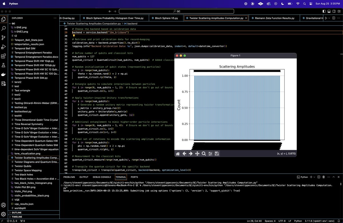
The computed scattering amplitudes are saved to a JSON and a histogram is plotted.

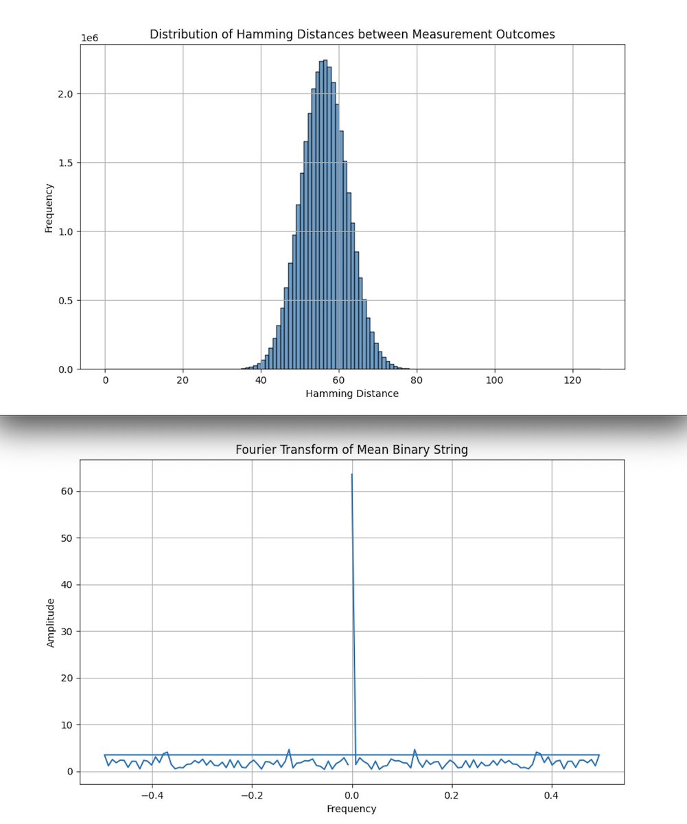
The histogram above (top) (code below) shows the distribution of Hamming distances between all pairs of measurement outcomes from the quantum circuit.
Peak at Hamming Distance ~60:
The quantum results obtained exhibit a clear concentration around a Hamming distance of ~60, suggesting that the states produced by the quantum circuit are moderately similar rather than entirely random.
The bell-shaped distribution of Hamming distances aligns with the idea that scattering amplitudes, when represented in twistor space, are not uniformly distributed but instead have a structured and symmetric pattern. This pattern may reflect the algebraic curves that support the amplitudes in twistor space.
Classical predictions for scattering amplitudes derived from twistor theory have shown that these amplitudes can often be simplified compared to their traditional formulations in quantum field theory. For example, Witten’s formulation of twistor string theory demonstrated that scattering amplitudes in twistor space exhibit high simplicity. These amplitudes are supported on algebraic curves, suggesting a deep connection between the geometry of twistor space and the physical scattering processes. This leads to a more compact and symmetric representation of amplitudes, often expressed in terms of Grassmannian residue formulas, polytopes, and the amplituhedron in twistor space.
The Fourier Transform of the mean binary string above (bottom) (code below) reveals a prominent spike at the zero frequency (DC component) and relatively low amplitudes across all other frequencies. This indicates that there is a strong constant component in the mean binary string, with very little variation in periodic components.
The significant spike at zero frequency suggests that the mean binary string has a strong constant value, indicating that most of the bits in the mean string are close to a constant value (either mostly 0s or mostly 1s). This could imply that there is a high degree of consistency in the states that are being measured, reflecting an underlying structure or symmetry.
In the context of twistor scattering amplitudes, the absence of strong periodic signals could suggest that the quantum circuit is capturing the non-periodic, continuous aspects of the scattering process. Twistor theory often simplifies scattering amplitudes by mapping complex interactions to geometrically simple objects in twistor space, but the underlying structure might not be periodic.

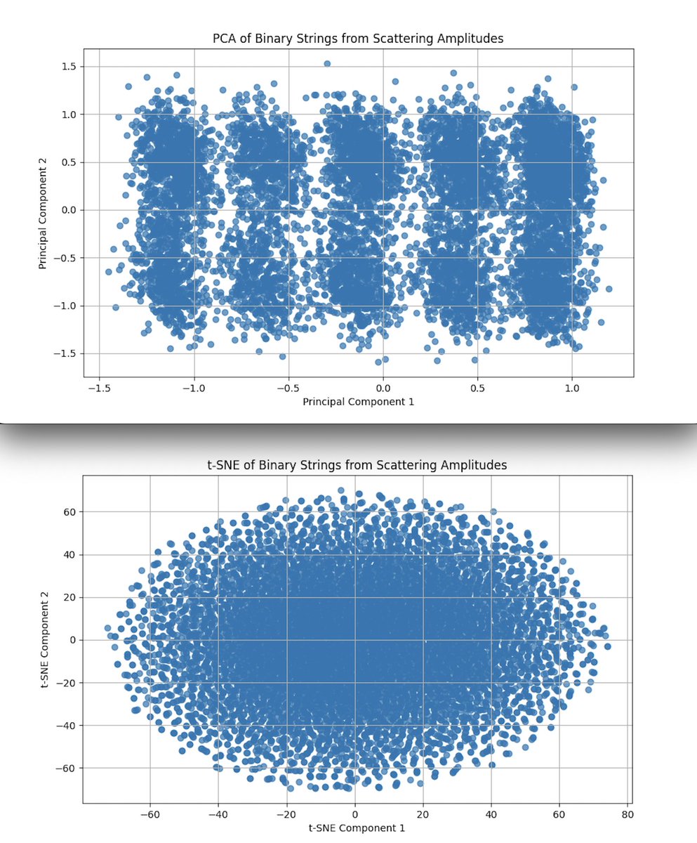
The PCA plot above (top) (code below) reveals that the binary strings cluster into distinct groups along the principal components, with noticeable gaps between these clusters.
The clustering observed in the PCA may indicate that the quantum circuit is sampling from distinct regions of the state space, possibly corresponding to different scattering events or configurations in twistor space. The separation of clusters suggests that the circuit outputs are not uniformly random but exhibit structured patterns, which aligns with the idea that twistor-inspired quantum circuits explore well defined regions of the state space.
The t-SNE plot above (bottom) (code below) shows a more continuous distribution without distinct clusters, forming an oval shaped distribution.
While t-SNE is sensitive to local similarities, the lack of distinct clustering in this plot suggests that, on a finer scale, the binary strings are more evenly distributed. This could indicate that while PCA reveals macro structure (global patterns), the quantum states are more uniformly spread when viewed through the lens of local similarities. This uniformity may suggest that the circuit captures a broader range of scattering events, each with subtle differences, which is consistent with the high complexity and variation expected in twistor scattering amplitudes.

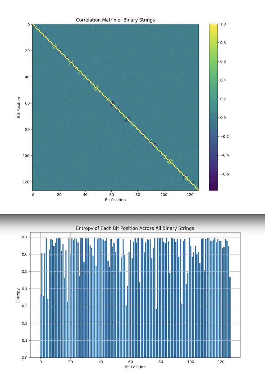
The Correlation Matrix of Binary Strings above (top) (code below) shows strong diagonal dominance, with relatively low off-diagonal correlations. The strong diagonal suggests that each bit is largely independent of the others, which is typical for high entropy, complex quantum systems. The few areas of off diagonal correlation might indicate interactions between specific qubits, possibly linked to the structure of the scattering amplitudes. The overall low correlation between most bit positions suggests that the quantum states do not exhibit simple, pairwise correlations but rather reflect a more intricate structure.
Lastly, the Entropy Plot above (bottom) (code below) shows that most bit positions have high entropy, with a few positions having slightly lower values. High entropy across most bit positions indicates that the bits are highly variable and not overly constrained, which aligns with the expected complexity of twistor-based scattering processes. The lower entropy in some positions might point to specific bits being more deterministic.
Entropy of Hamming distances: 3.1998136310587184
Total palindromic strings found: 0
The entropy of the Hamming distances is approximately 3.2, indicating a moderate spread of distances. This moderate entropy suggests that while there is some diversity in the Hamming distances (reflecting variation in the quantum states), the distribution is not entirely random. This aligns with the earlier observations of structured patterns in the state space.
In the end, the results show that the quantum circuit is exploring structured regions of the state space, consistent with the complex, high-dimensional nature of twistor scattering amplitudes. The clustering observed in PCA, the broad distribution seen in t-SNE, and the high entropy across bit positions all suggest that the quantum circuit captures a wide variety of states with underlying structure. The lack of simple symmetries, such as palindromes, further supports the complexity of the twistor based model.
Code:
# imports
import numpy as np
from qiskit import QuantumCircuit, transpile
from qiskit_ibm_runtime import QiskitRuntimeService, Session, SamplerV2
from qiskit.circuit.library import UnitaryGate
from qiskit.visualization import plot_histogram
import json
import logging
import matplotlib.pyplot as plt
from datetime import datetime
from scipy.stats import unitary_group

# Setup logging
logging.basicConfig(level=logging. INFO, filename='scattering_amplitudes.log',
filemode='w', format='%(asctime)s - %(levelname)s - %(message)s')

# Function to serialize datetime objects
def datetime_converter(o):
if isinstance(o, datetime):
return o.isoformat()

# Initialize IBM Qiskit Runtime Service
service = QiskitRuntimeService(
channel='ibm_quantum',
instance='ibm-q/open/main',
token='YOUR_IBMQ_KEY_O-`'
)

# Choose the backend
backend = service.backend("ibm_brisbane")

# Retrieve and print calibration data for record-keeping
calibration_data = backend. properties().to_dict()
logging. info("Backend Calibration Data: %s", json.dumps(calibration_data, indent=4, default=datetime_converter))

# Define number of qubits and classical bits
num_qubits = 127
quantum_circuit = QuantumCircuit(num_qubits, num_qubits)  # Added classical bits for measurements

# Random initialization of qubit states (representing particles)
for i in range(num_qubits):
theta = np.random.rand() * 2 * np.pi
quantum_circuit.ry(theta, i)

# Entangle qubits to simulate interactions between particles
for i in range(0, num_qubits - 1, 2):  # Ensure we don't go out of bounds
quantum_circuit.cx(i, i+1)

# Apply twistor Unitary transformations
for i in range(num_qubits):
# Generate a random unitary matrix representing twistor transformations
u_matrix = unitary_group.rvs(2)
unitary_gate = UnitaryGate(u_matrix)
quantum_circuit.append(unitary_gate, [i])

# Additional entanglement to mimic higher order particle interactions
for i in range(0, num_qubits - 3, 4):  # Ensure we don't go out of bounds
quantum_circuit.cx(i, i+2)
quantum_circuit.cx(i+1, i+3)

# Final set of rotations to encode the scattering amplitude information
for i in range(num_qubits):
phi = np.random.rand() * 2 * np.pi
quantum_circuit.rz(phi, i)

# Measurement to the classical bits
quantum_circuit.measure(range(num_qubits), range(num_qubits))

# Transpile the quantum circuit
transpiled_circuit = transpile(quantum_circuit, backend=backend, optimization_level=3)

# Log transpiled circuit depth and gate count
logging. info("Transpiled Circuit Depth: %d", transpiled_circuit.depth())
logging. info("Transpiled Circuit Gate Count: %s", transpiled_circuit.count_ops())

# Execution on backend with SamplerV2
with Session(service=service, backend=backend) as session:
sampler = SamplerV2(session=session)
# Run the circuit
job = sampler. run([transpiled_circuit], shots=8192)
job_result = job.result()
# Retrieve the classical register name
classical_register = quantum_circuit.cregs[0].name
# Extract counts for the first (and only) pub result
pub_result = job_result[0].data[classical_register].get_counts()

# Save the results to JSON
results_data = {

"raw_counts": pub_result
}
file_path = '/Users/Documents/scattering_amplitudes_result.json'
with open(file_path, 'w') as f:
json.dump(results_data, f, indent=4)
# Plotting the results for analysis
plot_histogram(pub_result)
plt.title("Scattering Amplitudes")

plt.savefig('/Users/Documents/scattering_amplitudes_histogram.png')
plt. show()

////////////////////////////////////////////////////////////////

Code for Hamming Distances Visual from Run Data
import json
import matplotlib.pyplot as plt
from itertools import combinations
from scipy.spatial.distance import hamming
import numpy as np

# Load the results JSON file
file_path = '/Users/Documents/scattering_amplitudes_result.json'
with open(file_path) as f:
    results_data = json.load(f)

# Extract the binary strings (keys) from the raw counts
binary_strings = list(results_data['raw_counts'].keys())

# Convert binary strings to arrays of integers
binary_arrays = [np.array(list(map(int, list(binary_string)))) for binary_string in binary_strings]

# Calculate Hamming distances between all pairs of binary strings
hamming_distances = [
    hamming(pair[0], pair[1]) * len(binary_arrays[0])  # Convert normalized distance to absolute number of differing bits
    for pair in combinations(binary_arrays, 2)
]

# Plot the histogram of Hamming distances
plt.figure(figsize=(10, 6))
plt.hist(hamming_distances, bins=range(0, len(binary_arrays[0]) + 1), edgecolor='black', alpha=0.7)
plt.title('Distribution of Hamming Distances between Measurement Outcomes')
plt.xlabel('Hamming Distance')
plt.ylabel('Frequency')
plt.grid(True)
plt.savefig('/Users/steventippeconnic/Documents/QC/hamming_distance_distribution.png')  # Save the plot
plt. show()

/////////////////////////////////////////////////////////////////

Code for the Fourier Transform of the mean binary string Visual with Run Data
import json
import numpy as np
import matplotlib.pyplot as plt

# Load the results JSON file
file_path = '/Users/Documents/scattering_amplitudes_result.json'
with open(file_path) as f:
    results_data = json.load(f)

# Extract the binary strings (keys) from the raw counts
binary_strings = list(results_data['raw_counts'].keys())

# Convert binary strings to arrays of integers
binary_arrays = np.array([list(map(int, list(binary_string))) for binary_string in binary_strings])

# Compute the mean binary string
mean_binary_array = np.mean(binary_arrays, axis=0)

# Perform Fourier transform on the mean binary array
fourier_transform = np.fft.fft(mean_binary_array)
frequencies = np.fft.fftfreq(len(mean_binary_array))

# Plot the Fourier Transform results
plt.figure(figsize=(10, 6))
plt.plot(frequencies, np.abs(fourier_transform))
plt.title('Fourier Transform of Mean Binary String')
plt.xlabel('Frequency')
plt.ylabel('Amplitude')
plt.grid(True)
plt.savefig('/Users/steventippeconnic/Documents/QC/fourier_scattering_amplitudes.png')
plt. show()

/////////////////////////////////////////////////////////////////

Code for Principal Component Analysis (PCA) Visual from Run Data
import json
import numpy as np
import matplotlib.pyplot as plt
from sklearn.decomposition import PCA

# Load the results JSON file
file_path = '/Users/Documents/scattering_amplitudes_result.json'
with open(file_path) as f:
results_data = json.load(f)

# Extract the binary strings (keys) from the raw counts
binary_strings = list(results_data['raw_counts'].keys())

# Convert binary strings to arrays of integers
binary_arrays = np.array([list(map(int, list(binary_string))) for binary_string in binary_strings])

# Perform PCA
pca = PCA(n_components=2)
principal_components = pca. fit_transform(binary_arrays)

# Plot the results
plt.figure(figsize=(10, 6))
plt.scatter(principal_components[:, 0], principal_components[:, 1], alpha=0.7)
plt.title('PCA of Binary Strings from Scattering Amplitudes')
plt.xlabel('Principal Component 1')
plt.ylabel('Principal Component 2')
plt.grid(True)
plt.savefig('/Users/steventippeconnic/Documents/QC/pca_scattering_amplitudes.png')
plt. show()

///////////////////////////////////////////////////////////////

Code for t-SNE (t-Distributed Stochastic Neighbor Embedding) Visual from Run Data
import json
import numpy as np
import matplotlib.pyplot as plt
from sklearn.manifold import TSNE

# Load the results JSON file
file_path = '/Users/Documents/scattering_amplitudes_result.json'
with open(file_path) as f:
    results_data = json.load(f)

# Extract the binary strings (keys) from the raw counts
binary_strings = list(results_data['raw_counts'].keys())

# Convert binary strings to arrays of integers
binary_arrays = np.array([list(map(int, list(binary_string))) for binary_string in binary_strings])

# Perform t-SNE
tsne = TSNE(n_components=2, random_state=42)
tsne_results = tsne. fit_transform(binary_arrays)

# Plot the results
plt.figure(figsize=(10, 6))
plt.scatter(tsne_results[:, 0], tsne_results[:, 1], alpha=0.7)
plt.title('t-SNE of Binary Strings from Scattering Amplitudes')
plt.xlabel('t-SNE Component 1')
plt.ylabel('t-SNE Component 2')
plt.grid(True)
plt.savefig('/Users/steventippeconnic/Documents/QC/tsne_scattering_amplitudes.png')
plt.s how()

///////////////////////////////////////////////////////////////

Code for Entropy Analysis Visual from Run Data
import json
import numpy as np
from scipy.stats import entropy
import matplotlib.pyplot as plt

# Load the results JSON file
file_path = '/Users/Documents/scattering_amplitudes_result.json'
with open(file_path) as f:
    results_data = json.load(f)

# Extract the binary strings (keys) from the raw counts
binary_strings = list(results_data['raw_counts'].keys())

# Convert binary strings to arrays of integers
binary_arrays = np.array([list(map(int, list(binary_string))) for binary_string in binary_strings])

# Calculate entropy for each bit position across all strings
bitwise_entropy = [entropy(np.bincount(binary_arrays[:, i])) for i in range(binary_arrays.shape[1])]

# Plot the entropy values
plt.figure(figsize=(10, 6))
plt. bar(range(len(bitwise_entropy)), bitwise_entropy)
plt.title('Entropy of Each Bit Position Across All Binary Strings')
plt.xlabel('Bit Position')
plt.ylabel('Entropy')
plt.grid(True)
plt.savefig('/Users/steventippeconnic/Documents/QC/entropy_scattering_amplitudes.png')
plt. show()

///////////////////////////////////////////////////////////////

Code for Correlation Analysis Visual from Run Data
import json
import numpy as np
import matplotlib.pyplot as plt

# Load the results JSON file
file_path = '/Users/Documents/scattering_amplitudes_result.json'
with open(file_path) as f:
    results_data = json.load(f)

# Extract the binary strings (keys) from the raw counts
binary_strings = list(results_data['raw_counts'].keys())

# Convert binary strings to arrays of integers
binary_arrays = np.array([list(map(int, list(binary_string))) for binary_string in binary_strings])

# Calculate the correlation matrix
correlation_matrix = np.corrcoef(binary_arrays, rowvar=False)

# Plot the correlation matrix
plt.figure(figsize=(10, 8))
plt.imshow(correlation_matrix, cmap='viridis', interpolation='none')
plt.colorbar()
plt.title('Correlation Matrix of Binary Strings')
plt.xlabel('Bit Position')
plt.ylabel('Bit Position')
plt.savefig('/Users/steventippeconnic/Documents/QC/correlation_scattering_amplitudes.png')
plt. show()

# End
