A Quantum-Based Secure Code Authentication App

This experiment explores the use of quantum computation to generate highly secure, time-sensitive authentication codes, similar to those used in traditional two-factor authentication (2FA) applications. By leveraging the quantum superposition and randomness properties of qubits, this creates a sequence of unique codes using IBM's 127-qubit quantum computer ibm_kyoto and Qiskit. The experiment uses the SamplerV2 primitive to run quantum circuits, retrieve measurement outcomes, and hash (SHA-256) the most probable bitstring to produce a 6-character secure code. An input algorithm requires the user to enter the most recent quantum-generated code for successful authentication, ensuring that only the latest secure quantum code can grant access.

Code Walkthrough

1. Initialization
We use IBM's 127-qubit quantum backend, ibm_kyoto, due to its high qubit count, allowing for maximum randomness in code generation.
2. Quantum Circuit Construction A quantum circuit qc is constructed with 127 qubits and 127 classical bits. This matches the maximum number of qubits on ibm_kyoto. To achieve maximum superposition, a Hadamard gate H is applied to each qubit:
H = 1/sqrt(2) * ​
(1, 1)
(​1, −1​)
This operation transforms each qubit into an equal superposition of ∣0⟩ and ∣1⟩:
H∣0⟩ = 1/sqrt(2) * ​(∣0⟩ + ∣1⟩)
Each qubit is then measured, collapsing the superposition into one of the basis states (either ∣0⟩ or ∣1⟩). The measurement outcomes are stored in the corresponding classical bits.
4. Quantum Execution
A session is opened with the IBM Quantum service using SamplerV2, ensuring that the circuit execution is performed in a controlled environment.
The transpiled circuit is executed with 8192 shots to gather statistically significant results.
5. Data Retrieval
The measurement outcomes are retrieved, representing the frequency of each bitstring (a sequence of 127 binary values) across the 8192 shots. The bitstring with the highest occurrence probability is identified as the most probable bitstring.
The counts are specifically extracted from the classical register associated with the quantum circuit.
6. Secure Code Generation
The most probable bitstring is hashed using the SHA-256 hashing algorithm:
Secure Code = SHA-256(Bitstring) mod10^6
This hashing process transforms the 127-bit bitstring into a unique 6-character alphanumeric code. The modulus operation ensures the final code is limited to a manageable size for use in authentication. A new secure quantum code is generated every 3 seconds with a new run.
7. Code Authentication and User Interaction
The generated secure code is displayed, and the user is prompted to enter the latest quantum secure code for validation.
The entered code is compared against the generated code. A match results in a "SUCCESS" message, while a mismatch leads to a "FAILURE" message.
8. Data Recording and Visual
The generated codes and associated measurement counts (raw results) are saved to a JSON. The JSON structure includes the codes, timestamps, and the backend name.
The distribution of measurement outcomes from the last iteration is visualized using a histogram. This plot displays the frequency of different bitstrings, highlighting the most probable bitstring used for code generation.

Results:
Run 3 times
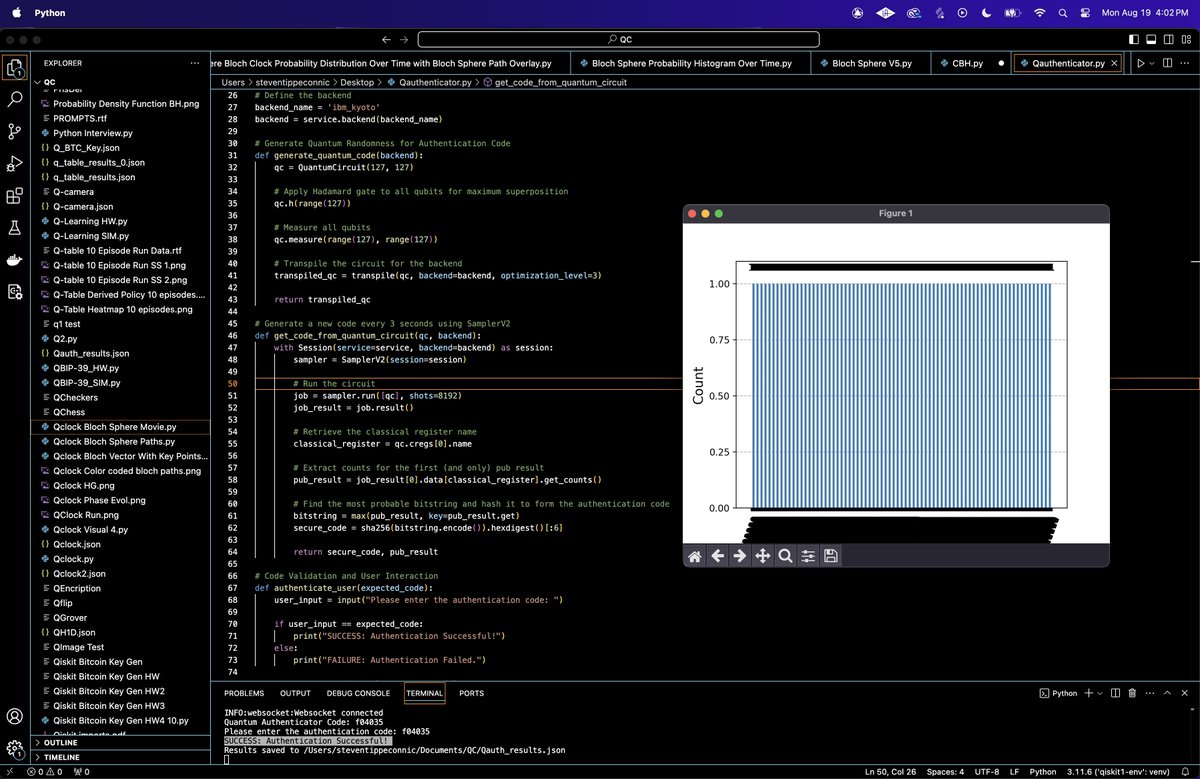
'Quantum Authenticator Code: 18d1d0
Quantum Authenticator Code: 06f9dc
Quantum Authenticator Code: f04035
Please enter the authentication code: f04035
SUCCESS: Authentication Successful!'
The experiment generated three quantum authentication codes: 18d1d0, 06f9dc, and f04035. The final code, f04035, was correctly entered for authentication, resulting in a "SUCCESS" message (on screenshot below).

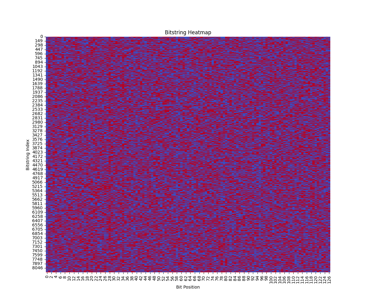
The heatmap above represents the binary values (0s and 1s) of bitstrings generated by the quantum circuit across all runs (code below). Each row corresponds to a unique bitstring, and each column represents a bit position in the 127-bit sequence. The color coding (blue for 0 and red for 1) helps quickly assess the distribution and patterns across the bitstrings.
The heatmap shows an even mix of blue and red across the bit positions, indicating a balanced distribution of 0s and 1s. This aligns with expectations given the application of Hadamard gates to each qubit, which should theoretically produce an equal probability for measuring 0 or 1 at each bit position.
The lack of any discernible patterns or clusters in the heatmap suggests a high degree of randomness in the generated bitstrings. This randomness is crucial for the security and unpredictability of the authentication codes.
With 8192 unique bitstrings, each 127 bits long, the heatmap's visual complexity underscores the vast potential for different outcomes. This large solution space is a fundamental reason why quantum based authentication can be more secure than classical methods.

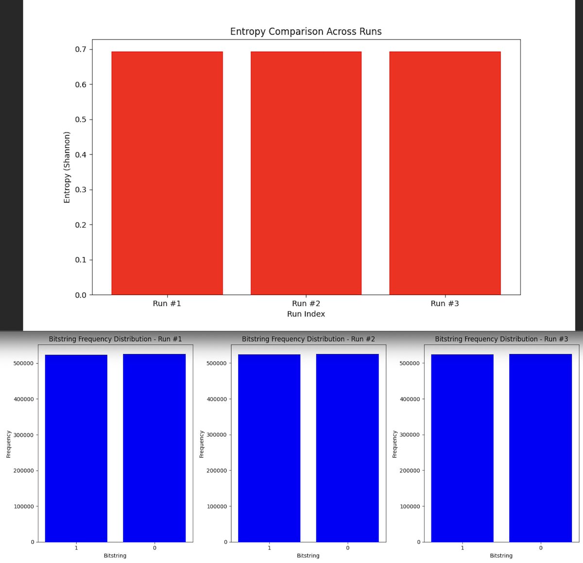
The entropy values across the three runs above (code below) are very similar, with all runs displaying an entropy close to 0.7 (Shannon). Entropy is a measure of randomness, and in the context of a quantum authenticator application, high entropy indicates that the bitstrings generated by the quantum circuit have a high degree of unpredictability. This is crucial for secure code generation, as the more random the output, the more difficult it is for an adversary to predict or replicate the generated authentication codes.
The bitstring frequency distribution above (code below) shows an almost equal number of '0' and '1' outcomes across all three runs. Exactly what we would expect from a balanced quantum system where each qubit has an equal probability of collapsing into the '0' or '1' state after measurement. The even distribution of '0's and '1's across the bitstrings indicates that the quantum circuit is functioning as intended, without bias towards any particular outcome. This balance is critical for the integrity of the quantum authenticator application, ensuring that the generated codes are uniformly distributed and do not exhibit any patterns that could be exploited.

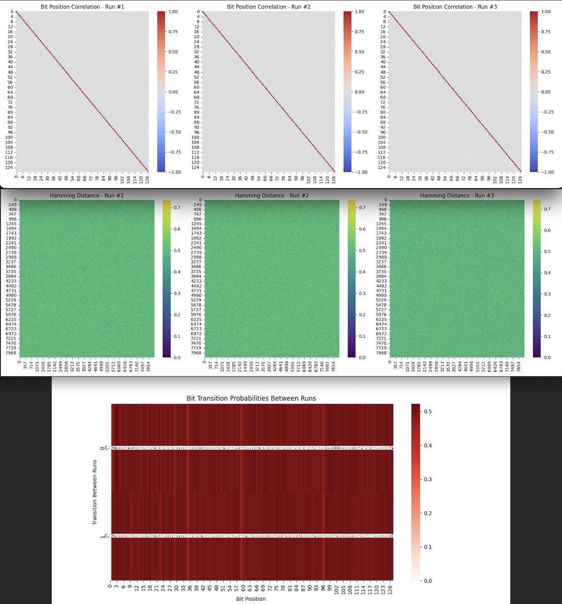
The bit position correlation heatmaps across the three runs above (code below) show that each bit position has a high correlation with itself (diagonal line of correlation = 1) and low to no correlation with other bit positions. This indicates that the bits are behaving independently from each other, which is desirable for a quantum authenticator application. If the bits were correlated, it could potentially allow an attacker to predict some bits based on the values of others, reducing the security of the generated code.
The Hamming distance heatmaps across the runs above (code below) display a uniform distribution of distances between bitstrings, with values hovering around the midpoint. This means that, on average, about half of the bits differ between any two given bitstrings. A uniform and high average Hamming distance between bitstrings is beneficial for a quantum authenticator. It ensures that each generated code is sufficiently different from others, making it challenging for attackers to guess subsequent codes based on previous ones.
The bit transition probability heatmap above shows that most bits have a low probability of transitioning between runs. This means that each bit is fairly stable, with a relatively low chance of flipping from 0 to 1 or vice versa. While stability is generally good for reliability, in the context of a quantum authenticator, some level of unpredictability (bit flipping) is necessary to ensure that each generated code is unique. The results suggest that the quantum system is functioning well, with enough variability to ensure that each authentication code is different from the previous one.
In the end, the experiment successfully demonstrated the use of a quantum based authenticator application by analyzing key metrics across multiple quantum runs. The results showed consistently high entropy, indicating strong randomness in the generated bitstrings, which is crucial for security. The bit position correlation heatmaps confirmed the independence of individual bits, ensuring unpredictability in the codes. The Hamming distance analysis revealed a uniform and sufficiently large distance between bitstrings, highlighting the uniqueness of each generated code. Additionally, the bit transition probabilities showed a balance between stability and variability, ensuring that while codes were distinct across runs, the underlying quantum system remained stable. This experiment shows the potential of quantum computing for secure authentication, with a reliable and secure method for generating unpredictable and unique quantum authentication codes.

Code:

# import
import numpy as np
import time
import json
import logging
from qiskit import QuantumCircuit, transpile
from qiskit_ibm_runtime import QiskitRuntimeService, Session, SamplerV2
from qiskit.visualization import plot_histogram
from hashlib import sha256
import matplotlib.pyplot as plt
from datetime import datetime

# Initialize logging
logging.basicConfig(level=logging. INFO)
logger = logging.getLogger(__name__)

# Input your IBM Quantum API key here
api_key = 'YOUR_IBM_KEY_O-`'

# Load IBMQ account
service = QiskitRuntimeService(
    channel='ibm_quantum',
    instance='ibm-q/open/main',
    token=api_key
)

# Define backend
backend_name = 'ibm_kyoto'
backend = service.backend(backend_name)

# Generate Quantum Randomness for Authentication Code
def generate_quantum_code(backend):
    qc = QuantumCircuit(127, 127)

    # Apply Hadamard gate to all qubits for maximum superposition
    qc.h(range(127))

    # Measure all qubits
    qc.measure(range(127), range(127))

    # Transpile the circuit for the backend
    transpiled_qc = transpile(qc, backend=backend, optimization_level=3)
    
    return transpiled_qc

# Generate a new code every 3 seconds using SamplerV2
def get_code_from_quantum_circuit(qc, backend):
    with Session(service=service, backend=backend) as session:
        sampler = SamplerV2(session=session)
        
        # Run the circuit
        job = sampler. run([qc], shots=8192)
        job_result = job.result()
        
        # Retrieve the classical register name
        classical_register = qc.cregs[0].name
        
        # Extract counts for the first (and only) pub result
        pub_result = job_result[0].data[classical_register].get_counts()
        
        # Find the most probable bitstring and hash it to form the authentication code
        bitstring = max(pub_result, key=pub_result.get)
        secure_code = sha256(bitstring.encode()).hexdigest()[:6]
        
        return secure_code, pub_result

# Code Validation and User Interaction
def authenticate_user(expected_code):
    user_input = input("Please enter the authentication code: ")
    
    if user_input == expected_code:
        print("SUCCESS: Authentication Successful!")
    else:
        print("FAILURE: Authentication Failed.")

# Record results to a JSON 
def record_results_to_json(data, file_path):
    with open(file_path, 'w') as file:
        json.dump(data, file, indent=4)

# Main Loop to generate and display quantum codes, with validation prompt after stopping
def quantum_authenticator_loop(backend, num_iterations=3, json_file_path='/Users/Documents/Qauth_results.json'):
    last_code = None
    all_pub_results = []
    try:
        for _ in range(num_iterations):
            qc = generate_quantum_code(backend)
            quantum_code, pub_result = get_code_from_quantum_circuit(qc, backend)
            print(f"Quantum Authenticator Code: {quantum_code}")
            last_code = quantum_code
            all_pub_results.append(pub_result)
            
            # Wait for 3 seconds before generating the next code
            time.sleep(3)
    except KeyboardInterrupt:
        print("\nLoop interrupted by user.")
    
    # After the loop or interruption, prompt for code validation
    if last_code:
        authenticate_user(last_code)
    else:
        print("No code was generated during this session.")
    
    # Record the generated codes and results to a JSON 
    results_data = {
        "quantum_codes": [last_code],
        "pub_results": all_pub_results,
        "timestamp": datetime. now().isoformat(),
        "backend": backend_name
    }
    record_results_to_json(results_data, json_file_path)
    print(f"Results saved to {json_file_path}")

    # Plotting the results
    if all_pub_results:
        plot_histogram(all_pub_results[-1])
        plt. show()

# Run the loop with a set number of iterations and save to JSON
quantum_authenticator_loop(backend, num_iterations=3, json_file_path='/Users/Documents/Qauth_results.json')

///////////////////////////////////////////////////////////

Code for Bitstring Heatmap Visual from Run Data
import json
import matplotlib.pyplot as plt
import numpy as np
import seaborn as sns

# Json Run File path
file_path = '/Users/Documents/Qauth_results.json'
with open(file_path, 'r') as f:
    data = json.load(f)

# Extract the bitstrings from the pub_results
bitstrings = [list(result.keys()) for result in data['pub_results']][0]

# Histogram of Bitstring Lengths
bitstring_lengths = [len(b) for b in bitstrings]

plt.figure(figsize=(10, 6))
plt.hist(bitstring_lengths, bins=range(126, 129), color='skyblue', edgecolor='black')
plt.title('Histogram of Bitstring Lengths')
plt.xlabel('Bitstring Length')
plt.ylabel('Frequency')
plt. show()

# Bitstring Frequencies (should all be 1)
frequencies = [1 for _ in bitstrings]  # Since each bitstring occurs exactly once

plt.figure(figsize=(10, 6))
plt.hist(frequencies, bins=range(1, 3), color='lightgreen', edgecolor='black')
plt.title('Distribution of Bitstring Frequencies')
plt.xlabel('Frequency')
plt.ylabel('Number of Bitstrings')
plt. show()

# Bitstring Heatmap
bitarray = np.array([[int(bit) for bit in b] for b in bitstrings])

plt.figure(figsize=(12, 10))
sns.heatmap(bitarray, cmap='coolwarm', cbar=False)
plt.title('Bitstring Heatmap')
plt.xlabel('Bit Position')
plt.ylabel('Bitstring Index')
plt. show()

///////////////////////////////////////////////////////////

Entropy Comparison Across Runs and Bitstring Frequency Distribution Visuals from Run Data
import json
import base64
import zlib
import numpy as np
import matplotlib.pyplot as plt
from collections import Counter
from scipy.stats import entropy
import seaborn as sns

# Json Run file paths
file_paths = [
    '/Users/Documents/Qauth Run Backend Results/Qauth Run Backend # 1 job-cv1w00gxrz3000899re0/Qauth Run Backend #1 job-cv1w00gxrz3000899re0-result.json',
    '/Users/Documents/Qauth Run Backend Results/Qauth Run Backend # 2 job-cv1wmtkhtzyg008q8dsg/Qauth Run Backend #2 job-cv1wmtkhtzyg008q8dsg-result.json',
    '/Users/Documents/Qauth Run Backend Results/Qauth Run Backend #3 job-cv1wsfx184p00089k0mg/Qauth Run Backend #3 job-cv1wsfx184p00089k0mg-result.json'
]

def decode_bitarray(encoded_data):
    # Decode the base64 and zlib encoded data
    decoded_data = zlib.decompress(base64.b64decode(encoded_data))
    bitstrings = [format(byte, '08b') for byte in decoded_data]
    return ''.join(bitstrings)

# Load the results from the three files
results = []
for file_path in file_paths:
    with open(file_path, 'r') as f:
        data = json.load(f)
        # Navigate through the structure to get to the bitstring data
        pub_results = data['__value__']['pub_results']
        for result in pub_results:
            bitarray_data = result['__value__']['data']['__value__']['fields']['c']['__value__']['array']['__value__']
            decoded_bitstring = decode_bitarray(bitarray_data)
            results.append(decoded_bitstring)

# 1. Bitstring Frequency Comparison
bitstring_counts_all = [Counter(result) for result in results]

# Plot the bitstring frequency distributions for the three runs
plt.figure(figsize=(15, 6))
for i, bitstring_counts in enumerate(bitstring_counts_all):
    plt.subplot(1, 3, i + 1)
    plt. bar(bitstring_counts.keys(), bitstring_counts.values(), color='blue')
    plt.title(f'Bitstring Frequency Distribution - Run #{i+1}')
    plt.xlabel('Bitstring')
    plt.ylabel('Frequency')

plt.tight_layout()
plt. show()

# 2. Entropy Comparison
bitstring_entropies = []

for bitstring_counts in bitstring_counts_all:
    probabilities = np.array(list(bitstring_counts.values())) / sum(bitstring_counts.values())
    bitstring_entropies.append(entropy(probabilities))

# Plot the entropy for each run
plt.figure(figsize=(10, 6))
plt. bar(range(1, 4), bitstring_entropies, color='red')
plt.title('Entropy Comparison Across Runs')
plt.xlabel('Run Index')
plt.ylabel('Entropy (Shannon)')
plt.xticks([1, 2, 3], ['Run #1', 'Run #2', 'Run #3'])
plt. show()

# 3. Bit-by-Bit Probability Comparison
bit_probabilities_all = []

for decoded_bitstring in results:
    bit_array = np.array([[int(bit) for bit in decoded_bitstring]])
    bit_probabilities = np.mean(bit_array, axis=0)
    bit_probabilities_all.append(bit_probabilities)

# Combine the bit probabilities into one array for comparison
bit_probabilities_combined = np.vstack(bit_probabilities_all)

# Plot the bit-by-bit probability heatmap comparison
plt.figure(figsize=(12, 8))
sns.heatmap(bit_probabilities_combined, cmap='coolwarm', cbar=True, annot=True, fmt=".2f")
plt.title('Bit-by-Bit Probability Comparison Across Runs')
plt.xlabel('Bit Position')
plt.ylabel('Run Index')
plt.yticks([0.5, 1.5, 2.5], ['Run #1', 'Run #2', 'Run #3'])
plt. show()

///////////////////////////////////////////////////////////

Bit Position Correlation Runs with Hamming Distances and Bit Transition Probabilities Between Run Visuals from Run Data
import json
import base64
import zlib
import numpy as np
import matplotlib.pyplot as plt
import seaborn as sns
from scipy.spatial.distance import pdist, squareform
from scipy.stats import entropy

# Json Run file paths
file_paths = [
    '/Users/Documents/Qauth Run Backend Results/Qauth Run Backend # 1 job-cv1w00gxrz3000899re0/Qauth Run Backend #1 job-cv1w00gxrz3000899re0-result.json',
    '/Users/Documents/Qauth Run Backend Results/Qauth Run Backend # 2 job-cv1wmtkhtzyg008q8dsg/Qauth Run Backend #2 job-cv1wmtkhtzyg008q8dsg-result.json',
    '/Users/Documents/Qauth Run Backend Results/Qauth Run Backend #3 job-cv1wsfx184p00089k0mg/Qauth Run Backend #3 job-cv1wsfx184p00089k0mg-result.json'
]

def decode_bitarray(encoded_data):
    # Decode the base64 and zlib encoded data
    decoded_data = zlib.decompress(base64.b64decode(encoded_data))
    bitstrings = [format(byte, '08b') for byte in decoded_data]
    return ''.join(bitstrings)

# Load and decode bitstrings from the results
results = []
for file_path in file_paths:
    with open(file_path, 'r') as f:
        data = json.load(f)
        pub_results = data['__value__']['pub_results']
        for result in pub_results:
            bitarray_data = result['__value__']['data']['__value__']['fields']['c']['__value__']['array']['__value__']
            decoded_bitstring = decode_bitarray(bitarray_data)
            results.append(decoded_bitstring)

# Set the bitstring length to 128
bitstring_length = 128

# Reshape the bit arrays into proper 2D arrays based on the bitstring length
bit_arrays = [np.array(list(map(int, decoded_bitstring))).reshape(-1, bitstring_length) for decoded_bitstring in results]

# Check the shape of each bit array 
for i, bit_array in enumerate(bit_arrays):
    print(f"New shape of bit array for Run #{i+1}: {bit_array.shape}")

# 1. Correlation Between Bit Positions
bit_correlations = [np.corrcoef(bit_array.T) for bit_array in bit_arrays]

plt.figure(figsize=(18, 6))
for i, corr in enumerate(bit_correlations):
    plt.subplot(1, 3, i + 1)
    sns.heatmap(corr, cmap='coolwarm', vmin=-1, vmax=1, cbar=True)
    plt.title(f'Bit Position Correlation - Run #{i+1}')
plt.tight_layout()
plt. show()

# 2. Hamming Distance Analysis
hamming_distances = [squareform(pdist(bit_array, metric='hamming')) for bit_array in bit_arrays]

plt.figure(figsize=(18, 6))
for i, hamming in enumerate(hamming_distances):
    plt.subplot(1, 3, i + 1)
    sns.heatmap(hamming, cmap='viridis', cbar=True)
    plt.title(f'Hamming Distance - Run #{i+1}')
plt.tight_layout()
plt. show()

# 3. Bitstring Transition Probability
transition_probabilities = []

for i in range(1, len(bit_arrays)):
    transitions = (bit_arrays[i] != bit_arrays[i - 1]).mean(axis=0)
    transition_probabilities.append(transitions)

transition_probabilities = np.vstack(transition_probabilities)

plt.figure(figsize=(12, 6))
sns.heatmap(transition_probabilities, cmap='Reds', annot=True, fmt=".2f")
plt.title('Bit Transition Probabilities Between Runs')
plt.xlabel('Bit Position')
plt.ylabel('Transition Between Runs')
plt. show()

# 4. Run Comparison Summary Plot
# Compare entropy and average Hamming distance for each run
entropies = [entropy(np.mean(bit_array, axis=0)) for bit_array in bit_arrays]
avg_hamming_distances = [np.mean(hamming) for hamming in hamming_distances]

fig, ax = plt.subplots(1, 2, figsize=(12, 6))

ax[0].bar(range(1, 4), entropies, color='blue')
ax[0].set_title('Entropy Comparison Across Runs')
ax[0].set_xlabel('Run Index')
ax[0].set_ylabel('Entropy')

ax[1].bar(range(1, 4), avg_hamming_distances, color='green')
ax[1].set_title('Average Hamming Distance Across Runs')
ax[1].set_xlabel('Run Index')
ax[1].set_ylabel('Average Hamming Distance')

plt.tight_layout()
plt. show()

# End