Quantum Timekeeping Using a Bloch Clock

This experiment using qiskit explores the concept of using a single qubit, a 'Bloch clock', to monitor the passage of quantum 'time' during a superposition collapse on IBM's 127-qubit quantum computer ibm_brisbine. The Bloch clock qubit evolves through a series of quantum gates, simulating the ticks of a clock while the remaining 126 qubits are prepared in a superposition state. These qubits are entangled with the Bloch clock and subjected to operations that eventually lead to the collapse of their superposition. The experiment is designed to visualize the evolution of the Bloch clock qubit on a Bloch sphere, providing insights into the dynamics of quantum state changes and their relation to the collapse of a superposition.

Code Walkthrough

1. Initialization of Quantum Registers
The experiment uses a quantum register with 127 qubits, denoted as q_0, q_1, …, q_126​.
A corresponding classical register is initialized to store the measurement results of the 127 qubits.
2. Bloch Clock Initialization
The first qubit q_0​ is designated as the Bloch clock qubit.
The Bloch clock qubit is placed in a superposition state using the Hadamard gate:
H∣0⟩ = 1/sqrt(2) * ​(∣0⟩ + ∣1⟩)
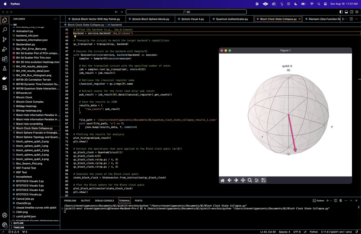
The circuit applies the Hadamard gate to q_0​, transforming its state into ∣+⟩, which lies on the equator of the Bloch sphere.
3. Superposition of the Remaining Qubits
Each of the remaining 126 qubits q_1, q_2, …, q_126​ is placed into a superposition state using Hadamard gates:
H∣0⟩ = 1/sqrt(2) * ​(∣0⟩ + ∣1⟩)
After applying the Hadamard gates, each qubit is in a superposition of ∣0⟩ and ∣1⟩, creating a highly entangled system across the entire register.
4. Entanglement with the Bloch Clock
The Bloch clock qubit q_0​ is entangled with each of the remaining 126 qubits using controlled-NOT gates. The operation for each qubit q_i is:
CNOT(q_0​, q_i​)
This operation entangles q_0 with all other qubits, meaning the state of q_0​ influences the state of the entire system.
5. Bloch Clock Evolution
The Bloch clock qubit undergoes a series of rotations around the X, Y, and Z axes to simulate the passage of quantum 'time':
RX​(θ) = e^(−i(θ/2)​X)
RY​(θ) = e^(−i(θ/2)Y)
RZ​(θ) = e^(−i(θ/2)​Z)
In this experiment, the angles for each rotation are set to π/4​:
RX​(π/4​​)
RY​(π/4​​)
RZ​(π/4​​)
These rotations move the Bloch clock qubit to different positions on the Bloch sphere, simulating the ticks of a clock.
6. Measurement of All Qubits
All 127 qubits are measured in the computational basis {∣0⟩, ∣1⟩}. The results of the measurement are stored in the classical register, collapsing the superposition of the 126 qubits and finalizing the state of the Bloch clock.
7. Transpilation and Execution on ibm_brisbane
The quantum circuit is transpiled to match the constraints of ibm_brisbane. The transpiled circuit is executed on IBM's 127-qubit quantum computer using the SamplerV2 primitive. The job is run with 8192 shots to gather sufficient data. The results are collected, and the counts for each measurement outcome are stored in a JSON.
8. Visualization
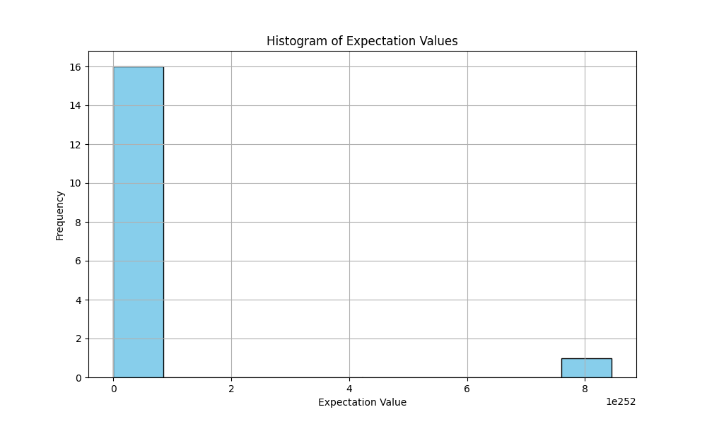
A histogram is generated to visualize the distribution of measurement outcomes across the 127 qubits. The final state of the Bloch clock qubit is shown separately to visualize its position on the Bloch sphere.

Results:

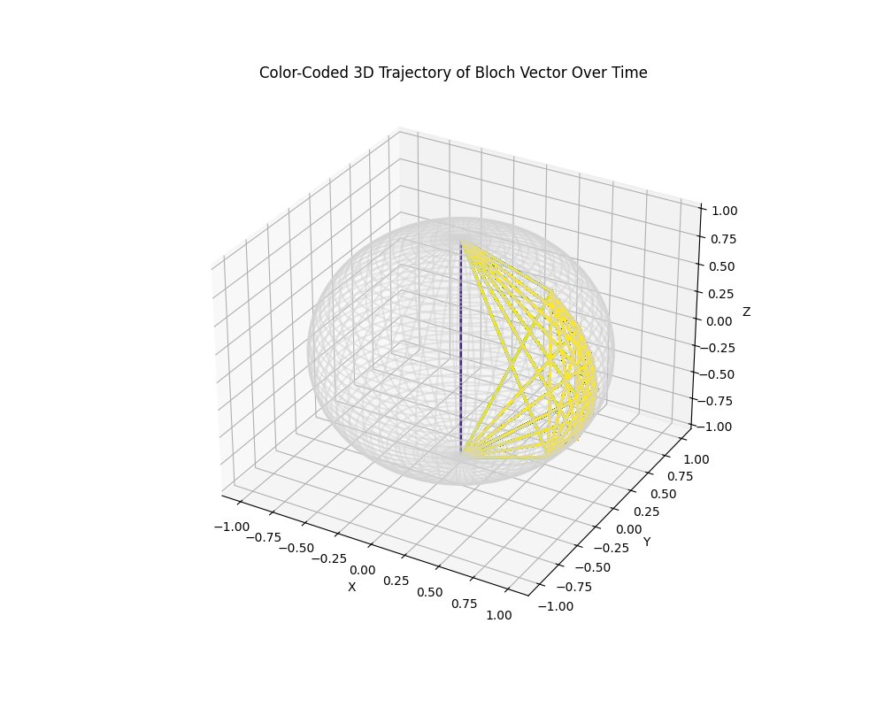
Number of paths counted: 126,142
The above result shows a densely packed trajectory on the Bloch sphere, with a total of 126,142 paths counted. The high number of paths indicates a significant amount of state transitions in the quantum clock. This suggests that the quantum system underwent many numerous small changes over time.

The heatmap above represents the collapse probabilities of qubit states as a function of the quantum clock's state, where the x-axis represents the qubit state index and the y-axis represents the quantum clock phase.
The heatmap visually represents how the state of the quantum system evolves as 'time' progresses according to the quantum clock. Each row corresponds to a different phase (or time step) of the quantum clock, and each column represents a possible qubit state. The relative uniformity and randomness of the heatmap suggest that as the quantum clock 'ticks,' the collapse probabilities do not follow a deterministic path but rather spread across many possible states.
The heatmap shows how, at each tick of the quantum clock, the system's state collapses into one of many possible states with certain probabilities. The randomness in the heatmap reflects the inherent probabilistic nature of quantum mechanics, where each measurement of the system yields different results.
As the quantum clock advances (moving down the y-axis), the system's evolution can be seen as the collapse probabilities changing across the x-axis. While these changes appear random, they still reflect the ticking of the clock as the system evolves probabilistically over time. The heatmap doesn’t show a clear 'signature' of time passing in the classical sense. Instead, it reflects the quantum clock’s function of evenly distributing the system's possible outcomes over time. The heatmap can be used to track the progression of quantum time by observing how the distribution of collapse probabilities evolves as the clock ticks. Even if the evolution appears random, the fact that it changes with each tick reflects the passage of 'time' within the quantum system.

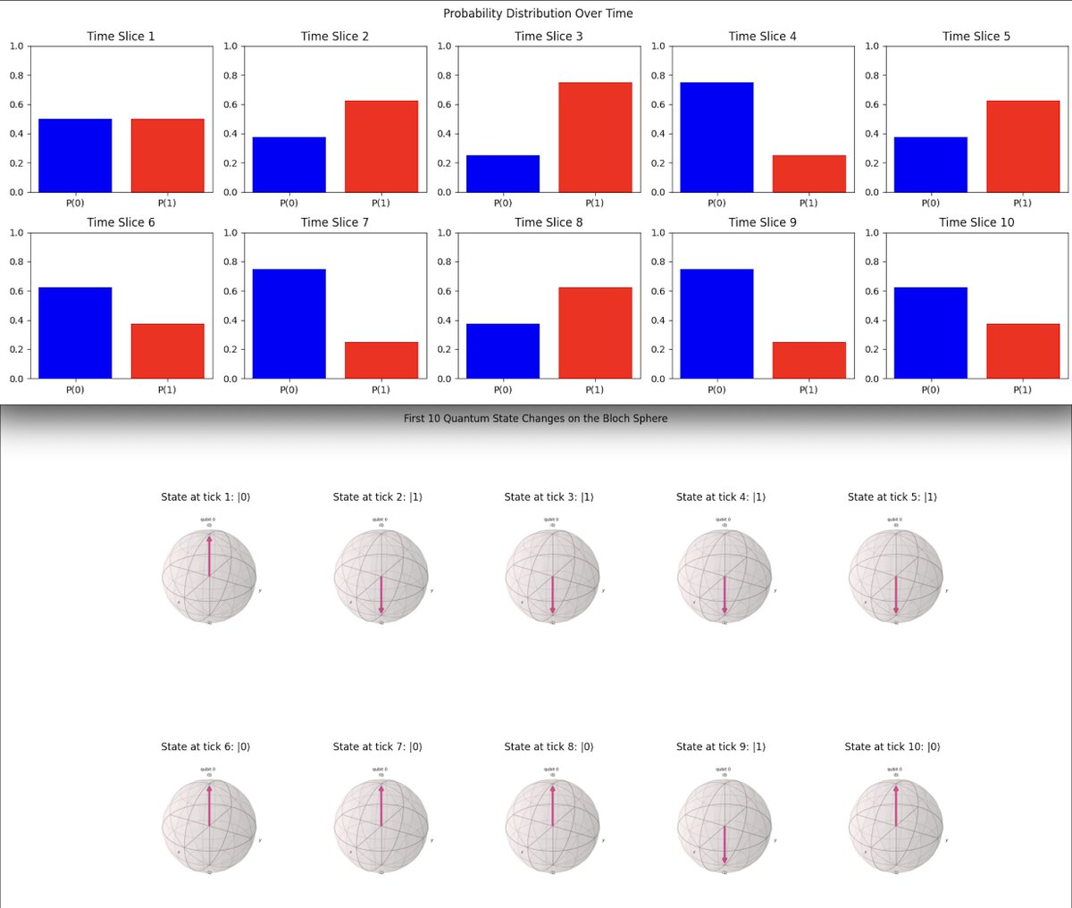
Probability Distribution Over Time Visual (Top)
The visualization above (top) shows the evolution of the probability distribution for measuring the qubit in the ∣0⟩ and ∣1⟩ states over time.
Initial Distribution (Time Slice 1)
In the first time slice, we observe that the probabilities for ∣0⟩ and ∣1⟩ are almost equal, with ∣0⟩ being slightly more probable. This indicates that at the beginning of the quantum clock's evolution, the qubit is in a superposition state with no strong preference for collapsing into either ∣0⟩ or ∣1⟩.
Early Evolution (Time Slices 2 to 4)
In the second and third time slices, the probability of measuring the qubit in ∣1⟩ increases, while the probability of ∣0⟩ decreases. This suggests that as time progresses, the wave function starts to collapse toward the ∣1⟩ state. In the fourth time slice, there is a significant reversion, where the probability of ∣0⟩ becomes dominant again. This could indicate a temporary reversal in the collapse process.
Mid Evolution (Time Slices 5 to 7)
Time slices 5 and 6 show a clear dominance of the ∣0⟩ state, with a significant probability for ∣0⟩ and a reduced probability for ∣1⟩. This suggests that the wave function is now strongly favoring the ∣0⟩ state. By the 7th time slice, the probabilities start to stabilize, with ∣0⟩ remaining dominant but with less pronounced fluctuations compared to earlier slices.
Late Evolution (Time Slices 8 to 10)
In the later time slices, 8 to 10, there is a return to a higher probability for ∣1⟩, indicating that the wave function is collapsing back toward the ∣1⟩ state. The probabilities here fluctuate, but ∣1⟩ begins to dominate again.
The wave function does not collapse linearly, it fluctuates between states, reflecting the quantum state evolution. The fluctuations in probabilities between ∣0⟩ and ∣1⟩ suggest that the quantum clock is subject to various influences that temporarily shift the state probabilities before they stabilize. The final time slices indicate that the wave function is collapsing into the ∣1⟩ state.
First 10 Quantum State Changes in the Bloch Sphere Visual (Bottom)
The second image above (bottom) represents the first 10 quantum state changes on the Bloch sphere, generated from the experimental run data using the Bloch clock.
The visual shows an oscillation pattern between the quantum states |0⟩ and |1⟩. This oscillation is captured by the Bloch vector flipping between the north pole (|0⟩) and the south pole (|1⟩) of the Bloch sphere.
In the context of the Bloch clock experiment, each state transition represents a 'tick' of the quantum clock. As the qubit oscillates between |0⟩ and |1⟩, these ticks are recorded on the Bloch sphere. The consistent transitions suggest a regular 'timekeeping' mechanism where the qubit alternates between states, simulating a simple quantum clock's ticking behavior.
This visual shows how the Bloch clock tracks the qubit's state changes over time. The regular pattern observed provides a demonstration of the qubit's oscillatory behavior, which is crucial for understanding time evolution in quantum systems. By using the Bloch sphere, we can visually and intuitively grasp the qubit's state transitions and how these transitions relate to the concept of quantum timekeeping.
In the end, this 'Bloch Clock' experiment used a single qubit to measure quantum 'time', visualizing its state transitions on the Bloch sphere as it oscillated between |0⟩ and |1⟩. This qubit's oscillations served as the ticks of the quantum clock, marking the passage of time with a quantum state. Throughout the experiment, we recorded '126,142 paths', representing the probabilistic nature of quantum state evolution. These paths reflect the potential outcomes the qubit could have taken before its wave function collapsed into a definite state upon measurement. The visualization of the first 10 state changes on the Bloch sphere provided a clear illustration of this process, showing how the qubit transitions through its state space before collapsing.

Code:

# imports
import numpy as np
import json
from qiskit import QuantumCircuit, QuantumRegister, ClassicalRegister, transpile
from qiskit_ibm_runtime import QiskitRuntimeService, Session, SamplerV2
from qiskit.visualization import plot_histogram, plot_bloch_multivector
from qiskit.quantum_info import Statevector
import matplotlib.pyplot as plt

# Initialize quantum register
qr = QuantumRegister(127)  # 1 qubit for the Bloch clock, 126 qubits for the superposition
cr = ClassicalRegister(127)  # Classical register to store the results
qc = QuantumCircuit(qr, cr)

# Step 1: Initialize the Bloch clock qubit (qr[0])
qc.h(qr[0])  # Start the Bloch clock in superposition (|+> state)

# Step 2: Create a superposition state across the 126 qubits
for i in range(1, 127):
    qc.h(qr[i])  # Apply Hadamard gate to create superposition

# Step 3: Apply a quantum algorithm that will eventually lead to collapse
# Example: Entangling the Bloch clock with all other qubits
for i in range(1, 127):
    qc. cx(qr[0], qr[i])  # Entangle the Bloch clock with all other qubits

# Step 4: Evolve the Bloch clock through some quantum gates
qc.rx(np.pi / 4, qr[0])  # Rotate Bloch clock around X-axis
qc.ry(np.pi / 4, qr[0])  # Rotate Bloch clock around Y-axis
qc.rz(np.pi / 4, qr[0])  # Rotate Bloch clock around Z-axis

# Step 5: Measure all qubits
qc.measure(qr, cr)

# Set up the IBMQ runtime service
service = QiskitRuntimeService(
    channel='ibm_quantum',
    instance='ibm-q/open/main',
    token='YOUR_IBMQ_KEY_O-`'  
)

# Define the backend 
backend = service.backend('ibm_brisbane')

# Transpile the circuit to match the target backend
qc_transpiled = transpile(qc, backend)

# Execute the circuit on the backend with SamplerV2
with Session(service=service, backend=backend) as session:
    sampler = SamplerV2(session=session)
    
    # Run the transpiled circuit with the specified number of shots
    job = sampler. run([qc_transpiled], shots=8192)
    job_result = job.result()
    
    # Retrieve the classical register name
    classical_register = qc.cregs[0].name

    # Extract counts for the first (and only) pub result
    pub_result = job_result[0].data[classical_register].get_counts()

    # Save the results to JSON
    results_data = {
        "raw_counts": pub_result
    }
    
    file_path = '/Users/Documents/quantum_clock_state_collapse_results_1.json'
    with open(file_path, 'w') as f:
        json.dump(results_data, f, indent=4)

# Plotting the results 
plot_histogram(pub_result)
plt. show()

# Extract the operations that were applied to the Bloch clock qubit (qr[0])
qc_bloch_clock = QuantumCircuit(1)
qc_bloch_clock.h(0)
qc_bloch_clock.rx(np.pi / 4, 0)
qc_bloch_clock.ry(np.pi / 4, 0)
qc_bloch_clock.rz(np.pi / 4, 0)

# Simulate the state of the Bloch clock qubit
state_bloch_clock = Statevector.from_instruction(qc_bloch_clock)

# Plot the Bloch sphere for the Bloch clock qubit
plot_bloch_multivector(state_bloch_clock)
plt. show()

////////////////////////////////////////////////////////////////

Code for Color-Coded 3D Trajectory of Bloch Vector Over Time with Path Counts
# imports
import json
import base64
import numpy as np
import matplotlib.pyplot as plt
from matplotlib import cm

# Path to JSON files
result_path = '/Users/Documents/job-cv13d1mg9ymg0081fz0g quantum_clock_state_collapse_results_1 Run Data/job-cv13d1mg9ymg0081fz0g-result.json'

# Load the results from JSON files
with open(result_path, 'r') as file:
    result_data = json.load(file)

# Extract and decode the bitstring data
bitstring_base64 = result_data["__value__"]["pub_results"][0]["__value__"]["data"]["__value__"]["fields"]["c0"]["__value__"]["array"]["__value__"]
bitstring_bytes = base64.b64decode(bitstring_base64)
bitstrings = [int(b) for b in bitstring_bytes]

# Convert the 8-bit values into binary strings
binary_bitstrings = [format(value, '08b') for value in bitstrings]

# Initialize lists to store the trajectory coordinates
x_coords = []
y_coords = []
z_coords = []

# Compute the Bloch vector for each measurement and store the coordinates
for binary_string in binary_bitstrings:
    prob_0 = binary_string.count('0') / 8
    theta = 2 * np.arccos(np.sqrt(prob_0))
    phi = 0  # assuming no phase for simplicity

    x_coords.append(np.sin(theta) * np.cos(phi))
    y_coords.append(np.sin(theta) * np.sin(phi))
    z_coords.append(np.cos(theta))

# Normalize the time steps for color mapping
time_steps = np.linspace(0, 1, len(x_coords))  # Normalize from 0 to 1 for colormap

# Set up the color map
colors = cm.viridis(time_steps)  # Using the 'viridis' colormap

# Plot the 3D trajectory with color-coded time evolution
fig = plt.figure(figsize=(10, 8))
ax = fig.add_subplot(111, projection='3d')

# Plot the Bloch sphere
u, v = np.mgrid[0:2*np.pi:100j, 0:np.pi:50j]
x = np.sin(v) * np.cos(u)
y = np.sin(v) * np.sin(u)
z = np.cos(v)
ax.plot_wireframe(x, y, z, color="lightgrey", alpha=0.5)

# Plot the trajectory, using color coding for time evolution
num_paths = 0
for i in range(1, len(x_coords)):
    ax.plot(x_coords[i-1:i+1], y_coords[i-1:i+1], z_coords[i-1:i+1], color=colors[i], linewidth=2)
    num_paths += 1  # Count each path segment

# Print the number of paths
print(f"Number of paths counted: {num_paths}")

# Setting labels and title
ax.set_xlabel('X')
ax.set_ylabel('Y')
ax.set_zlabel('Z')
ax.set_title("Color-Coded 3D Trajectory of Bloch Vector Over Time")

plt. show()

////////////////////////////////////////////////////////////////

Code for Heatmap of Collapse Probabilities vs. Quantum Clock State
# imports
import json
import zlib
import base64
import numpy as np
import matplotlib.pyplot as plt
import seaborn as sns

# Paths to JSON files
backend_results_path = '/Users/Documents/job-cv13d1mg9ymg0081fz0g quantum_clock_state_collapse_results_1 Run Data/job-cv13d1mg9ymg0081fz0g-result.json'

# Load JSON data 
with open(backend_results_path) as f:
    backend_results = json.load(f)

# Navigate to encoded data
encoded_data = backend_results['__value__']['pub_results'][0]['__value__']['data']['__value__']['fields']['c0']['__value__']['array']['__value__']

# Decode the base64-encoded and compressed data
compressed_data = base64.b64decode(encoded_data)
decompressed_data = zlib.decompress(compressed_data)

# Skip the header and load the numpy array
header_length = 128  # Assuming the header is 128 bytes long based on typical .npy headers
probabilities = np.frombuffer(decompressed_data[header_length:], dtype=np.uint8).reshape(8192, 16)

# Normalize the probabilities for visualization
probabilities = probabilities.astype(np.float64)
probabilities /= probabilities.sum(axis=1, keepdims=True)

# Create a heatmap
plt.figure(figsize=(12, 8))
sns.heatmap(probabilities, xticklabels=False, yticklabels=False, cmap='coolwarm')
plt.title("Heatmap of Collapse Probabilities vs. Quantum Clock State")
plt.xlabel("Qubit State Index")
plt.ylabel("Quantum Clock Phase")

# Save the heatmap
plt.savefig('/Users/Documents/job-cv13d1mg9ymg0081fz0g quantum_clock_state_collapse_results_1 Run Data/collapse_probabilities_heatmap.png')
plt. show()

////////////////////////////////////////////////////////////////

Code for Probability Distribution Over Time Visual
import json
import base64
import numpy as np
import matplotlib.pyplot as plt

# Path to JSON files
result_path = '/Users/Documents/job-cv13d1mg9ymg0081fz0g quantum_clock_state_collapse_results_1 Run Data/job-cv13d1mg9ymg0081fz0g-result.json'

# Load the results from JSON 
with open(result_path, 'r') as file:
    result_data = json.load(file)

# Extract and decode the bitstring data
bitstring_base64 = result_data["__value__"]["pub_results"][0]["__value__"]["data"]["__value__"]["fields"]["c0"]["__value__"]["array"]["__value__"]
bitstring_bytes = base64.b64decode(bitstring_base64)
bitstrings = [int(b) for b in bitstring_bytes]

# Convert the 8-bit values into binary strings
binary_bitstrings = [format(value, '08b') for value in bitstrings]

# Initialize lists to store the probabilities
probabilities_0 = []
probabilities_1 = []

# Compute the probabilities for each measurement
for binary_string in binary_bitstrings:
    prob_0 = binary_string.count('0') / 8
    prob_1 = 1 - prob_0  # Since prob_0 + prob_1 = 1
    
    probabilities_0.append(prob_0)
    probabilities_1.append(prob_1)

# Number of time slices 
time_slices = 10  
slice_indices = np.linspace(0, len(probabilities_0)-1, time_slices, dtype=int)

# Create subplots for histograms
fig, axes = plt.subplots(2, time_slices//2, figsize=(16, 6))

for i, ax in enumerate(axes.flat):
    index = slice_indices[i]
    ax. bar([0, 1], [probabilities_0[index], probabilities_1[index]], color=['blue', 'red'])
    ax.set_ylim(0, 1)
    ax.set_xticks([0, 1])
    ax.set_xticklabels(['P(0)', 'P(1)'])
    ax.set_title(f'Time Slice {i+1}')

plt.suptitle('Probability Distribution Over Time')
plt.tight_layout()
plt. show()

////////////////////////////////////////////////////////////////

Code for First 10 Quantum State Changes on the Bloch Sphere
import json
import base64
import numpy as np
from qiskit.visualization import plot_bloch_multivector
from qiskit.quantum_info import Statevector
import matplotlib.pyplot as plt
from PIL import Image
import io

# Load the JSON data
file_path = '/Users/Documents/job-cv13d1mg9ymg0081fz0g quantum_clock_state_collapse_results_1 Run Data/job-cv13d1mg9ymg0081fz0g-result.json'
with open(file_path, 'r') as file:
    data = json.load(file)

# Decode the base64 string
bitarray_base64 = data['__value__']['pub_results'][0]['__value__']['data']['__value__']['fields']['c0']['__value__']['array']['__value__']
bitarray_bytes = base64.b64decode(bitarray_base64)

# Convert to binary representation
bitstrings = [format(byte, '08b') for byte in bitarray_bytes]
bitstring = ''.join(bitstrings)[:len(bitarray_bytes) * 8]

# Initialize a list to store images
images = []

# Start with the |0⟩ state (north pole)
state = Statevector([1, 0])

# Collect the first 10 state changes and generate images
for i, bit in enumerate(bitstring[:10]):
    if bit == '0':
        state = Statevector([1, 0])  # |0⟩ state
    elif bit == '1':
        state = Statevector([0, 1])  # |1⟩ state
    
    # Generate the Bloch sphere plot and save it to an image in memory
    img_buf = io.BytesIO()
    plot_bloch_multivector(state).savefig(img_buf, format='png')
    img_buf.seek(0)
    images.append(Image. open(img_buf))

# Create a new figure for the grid of subplots
fig, axes = plt.subplots(2, 5, figsize=(20, 10))

# Arrange the images on the grid
for i, ax in enumerate(axes.flat):
    ax.imshow(images[i])
    ax.axis('off')
    ax.set_title(f'State at tick {i+1}: |{bitstring[i]}⟩')

plt.suptitle('First 10 Quantum State Changes on the Bloch Sphere')
plt. show()

# End