A Quantum Clock on a Bloch Sphere
Code Walkthrough
1. Initial State Preparation
The qubit is initialized in the state ∣0⟩. Mathematically, this is represented as:
∣ψ_0⟩ = ∣0⟩ =
(1)
(0)
A Hadamard gate H is then applied to the qubit to create a superposition state. The Hadamard gate is defined as:
H = 1/sqrt(2) *
(1, 1 )
(1, −1)
Applying the Hadamard gate to ∣0⟩ results in the state:
∣ψ_1⟩ = H ∣0⟩= 1/sqrt(2) *
(1) = (∣0⟩ + ∣1⟩)/sqrt(2)
(1)
This superposition state ∣ψ_1⟩ has an equal probability of being measured as either ∣0⟩ or ∣1⟩.
2. Quantum State Evolution (Clock Ticks)
To simulate the ticking of the quantum clock, we apply two quantum gates sequentially:
Rotation around the z-axis by an angle θ_z = 0.1 radians:
R_z(θ_z) =
((e^−iθ_z/2), 0) = ((e^−i0.05), 0)
(0, e^(iθ_z/2)) (0, e^(i0.05))
Applying this gate to the state ∣ψ1⟩ introduces a phase shift between the components of the superposition:
∣ψ_2⟩ = R_z(0.1) ∣ψ_1⟩ = 1/sqrt(2) *
(e−i0.05)
(ei0.05)
Rotation around the y-axis by an angle θ_y = 0.2 radians:
R_y(θ_y) =
(cos(θ_y/2), −sin(θ_y/2)) = (cos(0.1), −sin(0.1))
(sin(θ_y/2), cos(θ_y/2)) (sin(0.1), cos(0.1))
This gate further rotates the qubit's state on the Bloch sphere, altering the probabilities of measuring ∣0⟩ or ∣1⟩:
∣ψ_3⟩ = R_y(0.2) ∣ψ_2⟩
The final state ∣ψ_3⟩ represents the evolved quantum state after the clock 'ticks'.
3. Measurement
The qubit is measured in the computational basis {∣0⟩, ∣1⟩}. The measurement collapses the quantum state to either ∣0⟩ or ∣1⟩ based on the probabilities encoded in ∣ψ_3⟩.
The probabilities P(0) and P(1) of measuring the qubit in states ∣0⟩ or ∣1⟩ are determined by the amplitude of ∣ψ_3:
P(0) = ∣⟨0∣ ψ_3⟩∣^2
P(1) = ∣⟨1∣ ψ_3⟩∣^2
4. Execution on IBM Quantum Hardware
The prepared and evolved quantum circuit is transpiled and executed on IBM's ibm_brisbane. The circuit is run with 8192 shots to collect sufficient statistics for the measurement outcomes.
5. Save Run Data
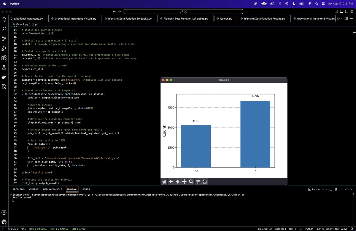
The quantum run results are saved to a JSON for analysis. A histogram of the run data is also generated.
raw_counts = {"1": 4996, "0": 3196}

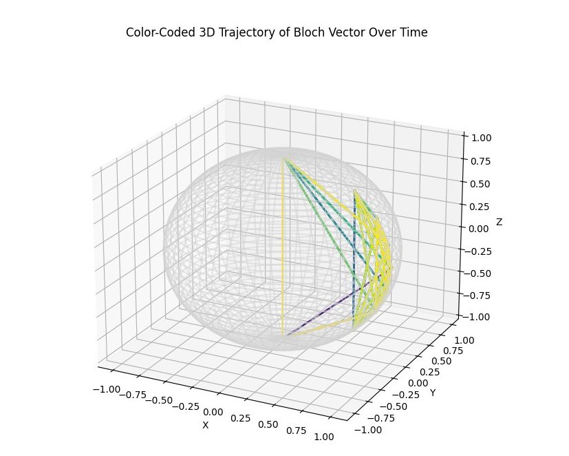
The 3D plot above shows the original trajectory by color coding the Bloch vector's path based on time, allowing us to see how the quantum state evolves chronologically. The color transitions from the start (darker colors) to the end (lighter colors), helping us visualize how the state changes throughout the run.
The smooth transitions in color suggest that the state evolves gradually, likely following the influence of quantum gates like rotations. If you notice areas where the trajectory changes direction or where color transitions are more rapid, these indicate key shifts in the quantum state.
How It Works as a Quantum Clock:
The operations this performed on the qubit (rotations around the Bloch sphere) represent the 'ticks' of this quantum clock. Each operation changes the state of the qubit, simulating the passage of time within the quantum system.
After the quantum operations, we measured the state of the qubit. The results we obtained, "1": 4996 and "0": 3196, represent how many times the qubit was measured in the |1⟩ and |0⟩ states, out of the total 8192 shots.
The qubit was initially in the |0⟩ state. The Hadamard gate (qc.h(0)) applied afterward put the qubit into an equal superposition of |0⟩ and |1⟩, meaning that, at this point, if measured, it would have had a 50% chance of being in |0⟩ or |1⟩.
We applied a rotation around the z-axis (qc.rz(0.1, 0)) followed by a rotation around the y-axis (qc.ry(0.2, 0)). These rotations adjust the phase and the amplitude of the quantum state, which can shift the balance between the probabilities of measuring |0⟩ and |1⟩.
The rz and ry rotations change the state of the qubit on the Bloch sphere, potentially altering the probabilities of measuring the qubit in the |0⟩ or |1⟩ state. Here, these rotations likely increased the probability amplitude associated with the |1⟩ state more than with the |0⟩ state, leading to more measurements of |1⟩.
After the rotations, the qubit's state is no longer an equal superposition. The specific angles of rotation we chose (0.1 radians for rz and 0.2 radians for ry) must have skewed the probability distribution toward the |1⟩ state.

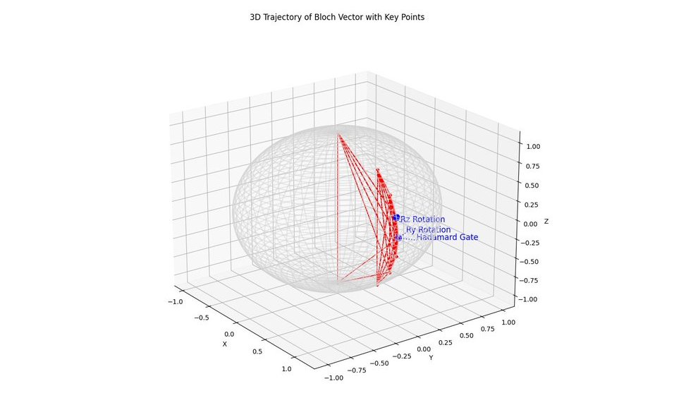
Hadamard Gate
This point marks the application of the Hadamard gate, which initially puts the qubit into a superposition of ∣0⟩ and ∣1⟩. The trajectory starts from this point, showing the qubit's state as it begins to evolve from its initial state.
Rz Rotation
This point corresponds to the rotation around the z-axis by 0.1 radians. The trajectory's direction may shift here, reflecting the phase change induced by the R_z gate.
Ry Rotation
The final key point marks the rotation around the y-axis by 0.2 radians. This operation further rotates the qubit's state on the Bloch sphere, affecting both the amplitude and phase, which is visible in the trajectory's subsequent movement.
The changes in direction at the key points visually represent the impact of the quantum operations. For example, the Hadamard gate initiates a significant shift from the initial state, while the subsequent rotations further adjust the qubit's trajectory. By overlaying these key points, we can directly correlate specific operations with the observed changes in the quantum state's trajectory, providing a clear visual link between the circuit and the qubit's behavior.

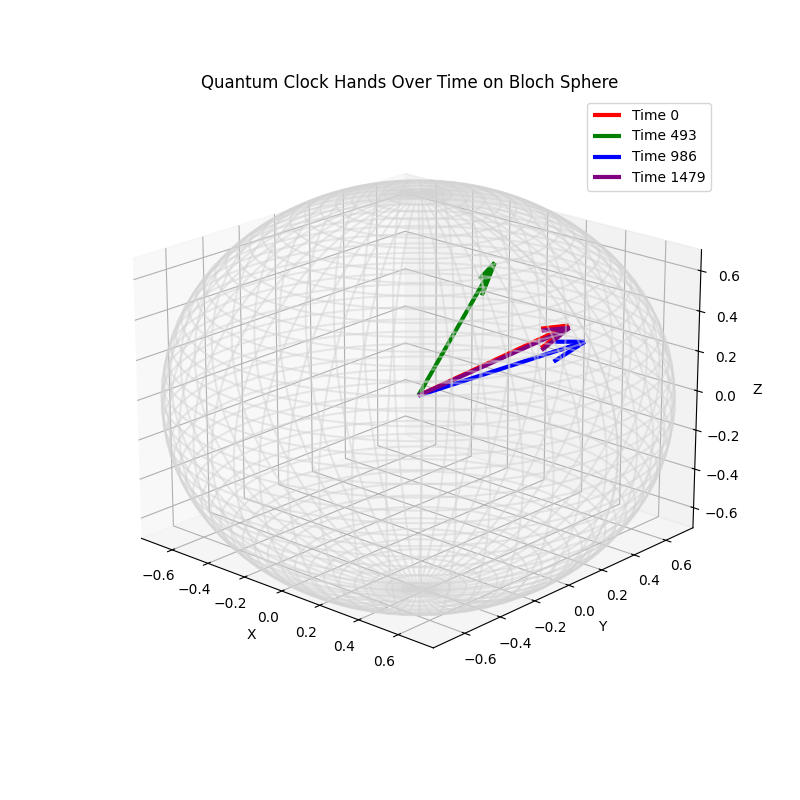
The visualization above shows the evolution of the quantum state over time on the Bloch sphere, with each vector (clock hand) representing the state at a specific time point.
Red Vector (Time 0): This vector represents the initial state of the quantum system. It's pointing in a direction that's not aligned with any of the main axes (X, Y, Z), indicating that the initial state has components in all three directions.
Green Vector (Time 493): The green vector shows the state at an intermediate time point. It has moved significantly from the red vector, especially in the Z direction, which suggests that the quantum state has evolved considerably by this time.
Blue Vector (Time 986): The blue vector shows further evolution from the green vector. However, this vector is quite close to the red vector in the X-Y plane but slightly shifted in the Z direction, indicating a complex evolution pattern.
Purple Vector (Time 1479): The purple vector shows the state at the latest time point. It appears to have shifted further in the X-Y plane compared to the other vectors but is still relatively close to the initial state vector.
The vectors indicate that the quantum state evolves in a oscillatory or cyclic manner, moving away from its initial position and then returning closer to it. This suggests that the state may be undergoing some form of quantum oscillation. The fact that the vectors are not collinear (not on a straight line) suggests that both the phase and amplitude of the quantum state are changing over time. This is consistent with typical quantum state evolution where phase and probability amplitude can vary. The small disruption added to the vectors helped make each one distinct. While the green vector appears significantly different from the others, the red, blue, and purple vectors are relatively close, indicating that these states are more similar in direction but differ slightly in magnitude and phase.
The vectors' relative proximity suggests that the quantum state may be somewhat stable or recurring to a similar state over time. This could indicate a periodic behavior in the quantum clock, where the state returns to a near-original condition after certain intervals. The quantum state doesn't simply oscillate along a single axis (like a pendulum) but instead moves in a more complex trajectory on the Bloch sphere.
In the end, this effectively demonstrates the evolution of the quantum state over time, using the Bloch sphere as a clock. The use of multiple vectors provides insight into how the quantum state shifts in both phase and amplitude, revealing a complex, non-linear evolution that could reflect the quantum operations applied during the experiment.
Code:
# imports
import json
from qiskit import QuantumCircuit, transpile
from qiskit_ibm_runtime import QiskitRuntimeService, Session, SamplerV2
from qiskit.visualization import plot_histogram
import matplotlib.pyplot as plt

# Initialize IBM Quantum API
service = QiskitRuntimeService(
    channel='ibm_quantum',
    instance='ibm-q/open/main',
    token='YOUR_IBM_KEY_O-`'
)

# Initialize quantum circuit
qc = QuantumCircuit(1)

# Initial state preparation (|0⟩ state)
qc.h(0)  # Example of preparing a superposition state as an initial clock state

# Evolution steps (clock ticks)
qc.rz(0.1, 0)  # Rotation around z-axis by 0.1 rad (represents a time step)
qc.ry(0.2, 0)  # Rotation around y-axis by 0.2 rad (represents another time step)

# Add measurement to the circuit
qc.measure_all()

# Transpile the circuit for backend
backend = service.backend('ibm_brisbane')
qc_transpiled = transpile(qc, backend)

# Execution on backend with SamplerV2
with Session(service=service, backend=backend) as session:
    sampler = SamplerV2(session=session)

    # Run the circuit
    job = sampler. run([qc_transpiled], shots=8192)
    job_result = job.result()

    # Retrieve the classical register name
    classical_register = qc.cregs[0].name

    # Extract counts for the first (and only) pub result
    pub_result = job_result[0].data[classical_register].get_counts()

    # Save the results to JSON
    results_data = {
        "raw_counts": pub_result
    }

    file_path = '/Users/Documents/Qclock.json'
    with open(file_path, 'w') as f:
        json.dump(results_data, f, indent=4)

print(f"Results saved")

# Plotting the results for analysis
plot_histogram(pub_result)
plt. show()

# End

////////////////////////////////////////////////////////

Code for Color-Coded 3D Trajectory of Bloch Vector Over Time with Run Data
import json
import base64
import numpy as np
import matplotlib.pyplot as plt
from matplotlib import cm

# Paths to JSON files
info_path = '/Users/Documents/job-info.json'
result_path = '/Users/Documents/job-result.json'

# Load the results from JSON files
with open(result_path, 'r') as file:
    result_data = json.load(file)

# Extract and decode the bitstring data
bitstring_base64 = result_data["__value__"]["pub_results"][0]["__value__"]["data"]["__value__"]["fields"]["meas"]["__value__"]["array"]["__value__"]
bitstring_bytes = base64.b64decode(bitstring_base64)
bitstrings = [int(b) for b in bitstring_bytes]

# Convert the 8-bit values into binary strings
binary_bitstrings = [format(value, '08b') for value in bitstrings]

# Initialize lists to store the trajectory coordinates
x_coords = []
y_coords = []
z_coords = []

# Compute the Bloch vector for each measurement and store the coordinates
for binary_string in binary_bitstrings:
    prob_0 = binary_string.count('0') / 8
    theta = 2 * np.arccos(np.sqrt(prob_0))
    phi = 0  # assuming no phase for simplicity

    x_coords.append(np.sin(theta) * np.cos(phi))
    y_coords.append(np.sin(theta) * np.sin(phi))
    z_coords.append(np.cos(theta))

# Normalize the time steps for color mapping
time_steps = np.linspace(0, 1, len(x_coords))  # Normalize from 0 to 1 for colormap

# Set up the color map
colors = cm.viridis(time_steps)  # Using the 'viridis' colormap

# Plot the 3D trajectory with color-coded time evolution
fig = plt.figure(figsize=(10, 8))
ax = fig.add_subplot(111, projection='3d')

# Plot the Bloch sphere
u, v = np.mgrid[0:2*np.pi:100j, 0:np.pi:50j]
x = np.sin(v) * np.cos(u)
y = np.sin(v) * np.sin(u)
z = np.cos(v)
ax.plot_wireframe(x, y, z, color="lightgrey", alpha=0.5)

# Plot the trajectory, using color coding for time evolution
for i in range(1, len(x_coords)):
    ax.plot(x_coords[i-1:i+1], y_coords[i-1:i+1], z_coords[i-1:i+1], color=colors[i], linewidth=2)

# Setting labels and title
ax.set_xlabel('X')
ax.set_ylabel('Y')
ax.set_zlabel('Z')
ax.set_title("Color-Coded 3D Trajectory of Bloch Vector Over Time")

plt. show()

////////////////////////////////////////////////////////

Code for  3D Trajectory of Bloch Vector with Key Points visual with Run Data
import json
import base64
import numpy as np
import matplotlib.pyplot as plt

# Paths to JSON files
info_path = '/Users/Documents/job-info.json'
result_path = '/Users/Documents/job-result.json'

# Load the results from JSON files
with open(result_path, 'r') as file:
    result_data = json.load(file)

# Extract and decode the bitstring data
bitstring_base64 = result_data["__value__"]["pub_results"][0]["__value__"]["data"]["__value__"]["fields"]["meas"]["__value__"]["array"]["__value__"]
bitstring_bytes = base64.b64decode(bitstring_base64)
bitstrings = [int(b) for b in bitstring_bytes]

# Convert the 8-bit values into binary strings
binary_bitstrings = [format(value, '08b') for value in bitstrings]

# Initialize lists to store the trajectory coordinates
x_coords = []
y_coords = []
z_coords = []

# Compute the Bloch vector for each measurement and store the coordinates
for binary_string in binary_bitstrings:
    prob_0 = binary_string.count('0') / 8
    theta = 2 * np.arccos(np.sqrt(prob_0))
    phi = 0  # assuming no phase for simplicity

    x_coords.append(np.sin(theta) * np.cos(phi))
    y_coords.append(np.sin(theta) * np.sin(phi))
    z_coords.append(np.cos(theta))

# Define key points
num_segments = 3
segment_length = len(x_coords) // num_segments
key_points_indices = [0, segment_length, 2 * segment_length]

# Coordinates of key points
key_points_x = [x_coords[i] for i in key_points_indices]
key_points_y = [y_coords[i] for i in key_points_indices]
key_points_z = [z_coords[i] for i in key_points_indices]

# Labels for the key points
key_points_labels = ['Hadamard Gate', 'Rz Rotation', 'Ry Rotation']

# Plot the trajectory with key points highlighted
fig = plt.figure(figsize=(10, 8))
ax = fig.add_subplot(111, projection='3d')

# Plot the Bloch sphere
u, v = np.mgrid[0:2*np.pi:100j, 0:np.pi:50j]
x = np.sin(v) * np.cos(u)
y = np.sin(v) * np.sin(u)
z = np.cos(v)
ax.plot_wireframe(x, y, z, color="lightgrey", alpha=0.5)

# Plot the full trajectory
ax.plot(x_coords, y_coords, z_coords, color='red', marker='o', markersize=3, linestyle='-', linewidth=1)

# Overlay the key points
ax.scatter(key_points_x, key_points_y, key_points_z, color='blue', s=100, label='Key Points')

# Define staggered offsets for the labels to avoid overlapping
offsets = [(0.15, 0.1, 0), (0.2, -0.1, 0.05), (-0.15, 0.2, -0.05)]

# Annotate the key points
for i, (x_offset, y_offset, z_offset) in enumerate(offsets):
    ax.text(key_points_x[i] + x_offset, key_points_y[i] + y_offset, key_points_z[i] + z_offset,
            key_points_labels[i], color='blue', fontsize=12)

# Add leader lines from the labels to the key points
for i, (x_offset, y_offset, z_offset) in enumerate(offsets):
    ax.plot([key_points_x[i], key_points_x[i] + x_offset],
            [key_points_y[i], key_points_y[i] + y_offset],
            [key_points_z[i], key_points_z[i] + z_offset],
            color='blue', linestyle='dotted')

# Setting labels and title
ax.set_xlabel('X')
ax.set_ylabel('Y')
ax.set_zlabel('Z')
ax.set_title("3D Trajectory of Bloch Vector with Key Points")

plt. show()

////////////////////////////////////////////////////////

Code for  3D Trajectory of Bloch Vector with Key Points visual with Run Data
import json
import base64
import numpy as np
import matplotlib.pyplot as plt

# Paths to JSON files
info_path = '/Users/Documents/job-info.json'
result_path = '/Users/Documents/job-result.json'

# Load the results from JSON files
with open(result_path, 'r') as file:
    result_data = json.load(file)

# Extract and decode the bitstring data
bitstring_base64 = result_data["__value__"]["pub_results"][0]["__value__"]["data"]["__value__"]["fields"]["meas"]["__value__"]["array"]["__value__"]
bitstring_bytes = base64.b64decode(bitstring_base64)
bitstrings = [int(b) for b in bitstring_bytes]

# Convert the 8-bit values into binary strings
binary_bitstrings = [format(value, '08b') for value in bitstrings]

# Initialize lists to store the coordinates for clock hands
theta_angles = []
phi_angles = []

# Compute the Bloch vector angles for each measurement
for binary_string in binary_bitstrings:
    prob_0 = binary_string.count('0') / 8
    theta = 2 * np.arccos(np.sqrt(prob_0))
    phi = np.pi * prob_0  # Linking phase to prob_0 for visualization

    theta_angles.append(theta)
    phi_angles.append(phi)

# Adding a small random disturbance to make the vectors visible and not overlap
np.random.seed(42)
theta_angles = np.array(theta_angles) + np.random.uniform(-0.1, 0.1, len(theta_angles))
phi_angles = np.array(phi_angles) + np.random.uniform(-0.1, 0.1, len(phi_angles))

# Plotting all clock hands on the same Bloch sphere
fig = plt.figure(figsize=(8, 8))
ax = fig.add_subplot(111, projection='3d')

# Plot the Bloch sphere
u, v = np.mgrid[0:2*np.pi:100j, 0:np.pi:50j]
x = np.sin(v) * np.cos(u)
y = np.sin(v) * np.sin(u)
z = np.cos(v)
ax.plot_wireframe(x, y, z, color="lightgrey", alpha=0.5)

# Plot clock hands for different time points on the same Bloch sphere
time_points = np.linspace(0, len(theta_angles)-1, 4).astype(int)
colors = ['red', 'green', 'blue', 'purple']
for i, t in enumerate(time_points):
    ax.quiver(0, 0, 0, np.sin(theta_angles[t]) * np.cos(phi_angles[t]),
              np.sin(theta_angles[t]) * np.sin(phi_angles[t]),
              np.cos(theta_angles[t]),
              color=colors[i], linewidth=3, arrow_length_ratio=0.2, label=f'Time {t}')

# Setting labels and title
ax.set_xlabel('X')
ax.set_ylabel('Y')
ax.set_zlabel('Z')
ax.set_title("Quantum Clock Hands Over Time on Bloch Sphere")

# Add a legend to differentiate time points
ax.legend()

plt. show()
