Quark-Antiquark Interaction Simulation Using IBMs 127-Qubit Quantum Computer Osaka
Code Walkthrough
1: Initialization
Start by initializing a quantum circuit with two qubits, each representing the quantum states of a quark and an antiquark.
Create a classical register with two bits to store the measurement results.
The quantum circuit is represented as:
qc = QuantumCircuit(2)
cr = ClassicalRegister(2)
2. Representation of Quark and Antiquark States
Place the qubits in superposition states to represent the quark and antiquark. This is done by applying Hadamard gates to both qubits.
The Hadamard gate H creates a superposition of the basis states ∣0⟩ and ∣1⟩ as:
H∣0⟩ = 1/sqrt(2) * (∣0⟩ + ∣1⟩)
After applying the Hadamard gate to both qubits, the combined state of the system is:
∣ψ_initial⟩ = 1/sqrt(2) * (∣00⟩ + ∣01⟩ + ∣10⟩ + ∣11⟩)
3. Defining the Quark-Antiquark Interaction
To simulate the interaction between the quark and antiquark, define a custom gate sequence. This sequence represents the transformation of the quark-antiquark pair into a meson. The sequence involves:
a. A controlled-NOT (CNOT) gate is applied where the quark qubit is the control, and the antiquark qubit is the target. The CNOT gate creates entanglement between the qubits, reflecting the interaction.
CNOT=
( 1, 0, 0, 0
0, 1, 0, 0
0, 0, 0, 1
0, 0, 1, 0 )
b. A Hadamard gate is applied to the quark qubit, further manipulating the superposition and entanglement.
H = 1/sqrt(2) * ( 1, 1
1, -1 )
c. A Pauli-X gate (or NOT gate) is applied to flip the state of the quark qubit.
X = ( 0, 1
1, 0 )
d. Another CNOT gate is applied, this time with the antiquark qubit as the control and the quark qubit as the target.
4. Measurement of the Quantum States
After defining the interaction, measure the final states of the qubits to observe the outcome of the quark-antiquark interaction. The measurement collapses the quantum superposition into classical states ∣00⟩, ∣01⟩, ∣10⟩, or ∣11⟩, with probabilities determined by the quantum gates applied.
5. Transpiling and Executing the Circuit
The quantum circuit is transpiled to optimize it for Osaka. The transpiled circuit is then executed using the SamplerV2 function to run the quantum circuit multiple times (8192 shots) and obtain measurement statistics.
6. Extracting Measurement Results
The measurement results are extracted from the job result. The counts of the measured states are obtained and stored for analysis. The measurement counts provide insight into the probabilities of the different outcomes of the quark-antiquark interaction. The measurement counts, along with other relevant information (backend used, job ID, execution status, etc), are saved to a JSON file for analysis.
7. Visualizing the Results
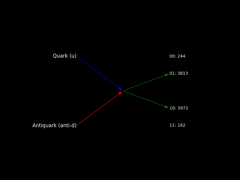
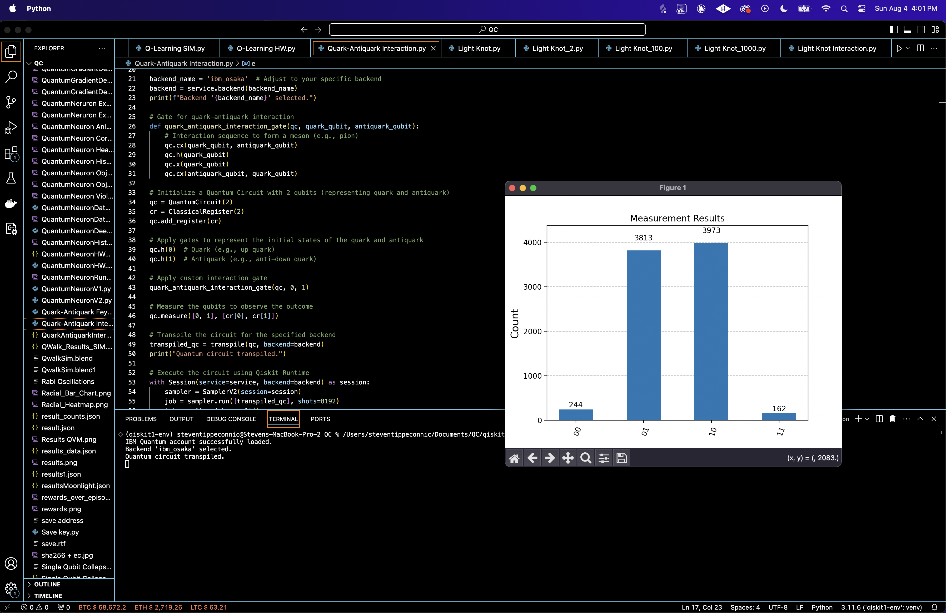
A histogram of the measurement results is generated to visualize the distribution of the different quantum states. Additionally, a Feynman-like diagram is created to provide an intuitive understanding of the quark-antiquark interaction and the possible outcomes. The Feynman-like diagram depicts the quark and antiquark as incoming lines, with the interaction vertex representing their interaction. The outgoing lines represent the possible resulting states, with their opacity indicating the relative probability of each state.

This Feynman-like diagram above visualizes the quark-antiquark interaction, with the outcome lines' opacities representing the relative probabilities of the quantum states. The states 10 and 01 have the most prominent lines, reflecting their higher probabilities, while the 11 and 00 states are much fainter, indicating their lower likelihood. From the run, we observe the following measurement counts: State '10': 3973 counts State '01': 3813 counts State '11': 162 counts State '00': 244 counts The outcomes 10 and 01 dominate, with nearly equal counts: 3973 and 3813. The states 11 and 00 are much less frequent, with only 162 and 244 counts. This distribution suggests that the quark-antiquark interaction predominantly results in one of two main states: 10 and 01. This could be interpreted as a meson forming with the quark and antiquark, with the quantum system collapsing into one of these likely states. The Hadamard gate and CNOT gates applied during the interaction phase of the circuit introduce entanglement and quantum interference. The outcomes 10 and 01 result from constructive interference of the amplitudes, making them more probable. The less probable states 11 and 00 likely result from destructive interference, which diminishes their probability amplitude, hence fewer occurrences are observed.

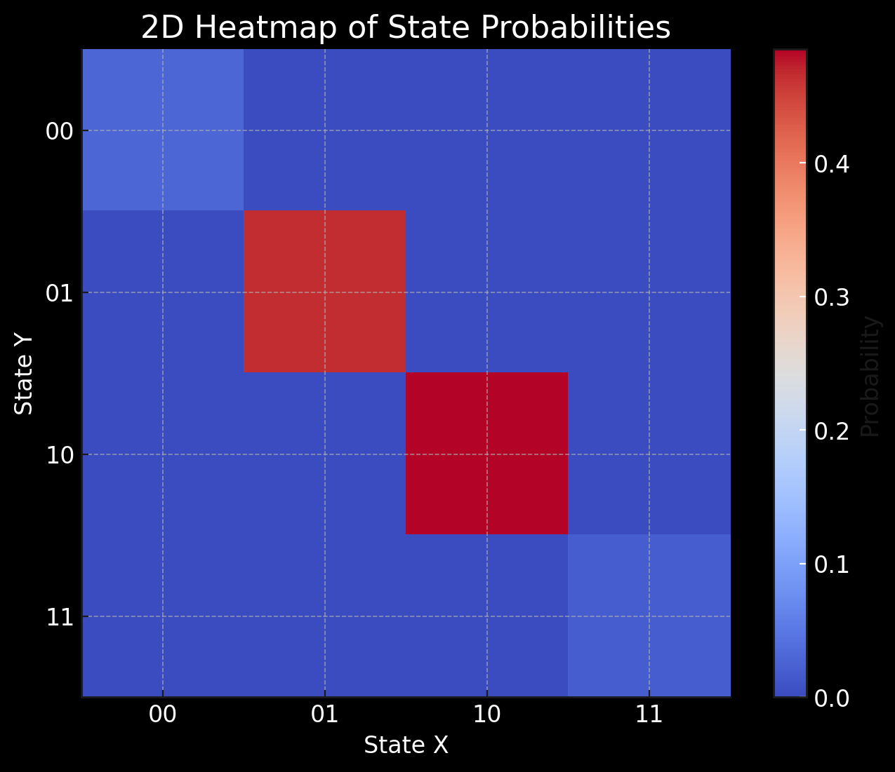
This heatmap above provides a top-down view of the probability distribution across the different quantum states. The states 10 and 01 have the highest probabilities (red), while the states 11 and 00 have much lower probabilities (blue).

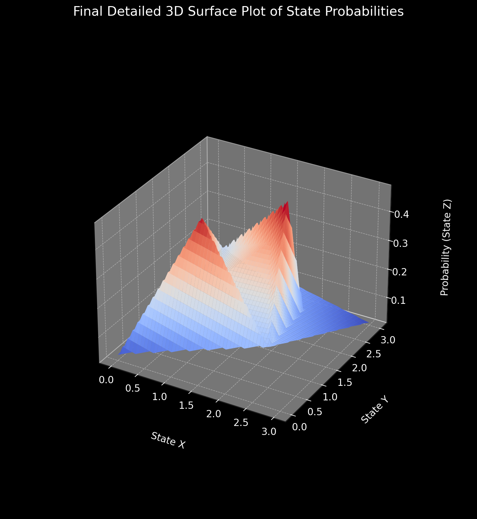
This 3D surface plot above visually represents the probability distribution across different quantum states derived from the experiment. The surface's peaks and valleys correspond to high and low probabilities, providing a clear, visual representation of the likelihood of each state. The X-Axis (State X) represents the discrete quantum states along one dimension. The Y-Axis (State Y) represents the same quantum states but aligned on another dimension. The Z-Axis (Probability - State Z) represents the probability associated with each quantum state.
In the end, this experiment successfully simulates the interaction between a quark and an antiquark using quantum computing. By applying specific quantum gates, the circuit abstractly represents the formation of a meson and observes the probabilistic nature of the resulting quantum states. The experiment highlights the power of quantum computing in modeling complex particle interactions through probabilities. The visualizations further enhance our view by depicting the interaction process reminiscent of Feynman diagrams. This approach can be extended to simulate other particle interactions (including my previous Exploring abstract Electron-Positron Annihilation on IBM's 127-Qubit Quantum Computer Osaka), offering a tool for exploring quantum and probabilistic phenomena.
Code:
# imports
from qiskit import QuantumCircuit, transpile, ClassicalRegister
from qiskit_ibm_runtime import QiskitRuntimeService, Session, SamplerV2
from qiskit.visualization import plot_histogram
import json
from datetime import datetime
import matplotlib.pyplot as plt

# IBM Quantum API key and backend setup
api_key = 'YOUR_IBM_API_KEY_O-`'  # Replace with your API key
QiskitRuntimeService. save_account(channel='ibm_quantum', token=api_key, overwrite=True)

# Account saved and loaded
try:
    service = QiskitRuntimeService(channel='ibm_quantum', token=api_key)
    print("IBM Quantum account successfully loaded.")
except Exception as e:
    print("Error loading IBM Quantum account:", str(e))
    exit()

backend_name = 'ibm_osaka'  # Adjust to backend
backend = service.backend(backend_name)
print(f"Backend '{backend_name}' selected.")

# Gate for quark-antiquark interaction
def quark_antiquark_interaction_gate(qc, quark_qubit, antiquark_qubit):
    # Interaction sequence to form a meson (e.g, pion)
    qc. cx(quark_qubit, antiquark_qubit)
    qc.h(quark_qubit)
    qc.x(quark_qubit)
    qc. cx(antiquark_qubit, quark_qubit)

# Initialize a Quantum Circuit with 2 qubits (representing quark and antiquark)
qc = QuantumCircuit(2)
cr = ClassicalRegister(2)
qc.add_register(cr)

# Apply gates to represent the initial states of the quark and antiquark
qc.h(0)  # Quark (e.g., up quark)
qc.h(1)  # Antiquark (e.g., anti-down quark)

# Apply custom interaction gate
quark_antiquark_interaction_gate(qc, 0, 1)

# Measure the qubits to observe the outcome
qc.measure([0, 1], [cr[0], cr[1]])

# Transpile the circuit
transpiled_qc = transpile(qc, backend=backend)
print("Quantum circuit transpiled.")

# Execute the circuit with Qiskit Runtime
with Session(service=service, backend=backend) as session:
    sampler = SamplerV2(session=session)
    job = sampler. run([transpiled_qc], shots=8192)
    job_result = job.result()

# Extract counts from the job result
counts = job_result[0].data[cr. name].get_counts()

# Save data to a JSON file
data = {
    'measurement_counts': counts,
    'backend': backend_name,
    'job_id': job.job_id(),
    'status': job.status(),
    'execution_date': datetime. now().strftime("%Y-%m-%d %H:%M:%S")
}
output_file = '/Users/Documents/QuarkAntiquarkInteraction.json'
with open(output_file, 'w') as f:
    json.dump(data, f, indent=4, default=str)

# Display histogram of measurement results with counts
plot_histogram(counts, title='Measurement Results', bar_labels=True)
plt. show()

# Feynman-like Diagram from Run Result Code
# imports
import json
import matplotlib.pyplot as plt
import numpy as np

# Load measurement counts from JSON
with open('/Users/Documents/QuarkAntiquarkInteraction.json', 'r') as file:
    measurement_counts = json.load(file)['measurement_counts']

# Define the figure for the Feynman-like diagram
fig, ax = plt.subplots(figsize=(8, 6))
ax.axis('off')  # Remove the axis as they are not needed
ax.set_xlim([0, 4])
ax.set_ylim([0, 4])

# Define positions for the particles and vertices in the diagram
quark_position = (1, 3)
antiquark_position = (1, 1)
interaction_vertex = (2, 2)
outcomes_positions = {
    '00': (3, 3),
    '01': (3, 2.5),
    '10': (3, 1.5),
    '11': (3, 1)
}

# Draw quark and antiquark lines to the interaction vertex
ax.annotate('', xy=interaction_vertex, xytext=quark_position,
            arrowprops=dict(facecolor='blue', shrink=0, width=2, headwidth=8))
ax.annotate('', xy=interaction_vertex, xytext=antiquark_position,
            arrowprops=dict(facecolor='red', shrink=0, width=2, headwidth=8))

# Label the quark and antiquark
ax.text(*quark_position, 'Quark (u)', ha='right', va='center', fontsize=12, color='white')
ax.text(*antiquark_position, 'Antiquark (anti-d)', ha='right', va='center', fontsize=12, color='white')

# Draw outcome lines and label them, using the counts as probability amplitudes
for state, position in outcomes_positions.items():
    opacity = measurement_counts[state] / max(measurement_counts.values())  # Opacity based on relative count
    ax.annotate('', xy=position, xytext=interaction_vertex,
                arrowprops=dict(facecolor='green', alpha=opacity, shrink=0, width=2, headwidth=8))
    ax.text(*position, f'{state}: {measurement_counts[state]}', ha='left', va='center', fontsize=10, color='white')

# Background color
fig.patch.set_facecolor('black')
ax.set_facecolor('black')

# Display the Feynman-like diagram
plt. show()

# End
