Optimizing a Quantum Neuron Using Gradient Descent on IBM Osaka

This experiment aims to implement and test a quantum version of a gradient descent algorithm on IBM's 127-qubit quantum computer Osaka using qiskit. The primary goal is to optimize a parameterized quantum circuit (simulating a quantum neuron) to minimize a specific objective function. This process involves iteratively adjusting the circuit parameters to achieve a desired expectation value.

Code Walkthrough

1. Initialization and Setup:
Define the backend as IBM Osaka.

2. Quantum Circuit Definition:
We construct a parameterized quantum circuit (quantum neuron) with one qubit and one classical bit.
The circuit includes:
A Hadamard gate to create superposition.
A parameterized rotation around the z-axis R_z * ​(θ)).
Another Hadamard gate.
Measurement of the qubit state.
We define the parameter θ as a Parameter object for optimization purposes.

3. Execution Function:
We create a function to execute the parameterized circuit on the backend.
We then bind the parameter θ to the circuit and transpile it for the specified backend with an optimization level of 3.
We use the Sampler from qiskit_ibm_runtime to run the circuit with 512 shots per run.
Then we extract and return the counts of measurement results from the quasi_dists in the results.

4. Objective Function:
First we define an objective function to minimize. The goal is to achieve an expectation value ⟨Z⟩ close to 1.
The expectation value ⟨Z⟩ is calculated as P(0) − P(1), where P(0) and P(1) are the probabilities of measuring the qubit in states '0' and '1', respectively.
The objective function is (⟨Z⟩ − 1)^2.

5. Gradient Calculation:
We implement a numerical gradient calculation using finite differences to estimate the gradient of the objective function with respect to the parameter
Then we define a small perturbation ϵ and compute the gradient as the difference in the objective function values at θ and θ + ϵ.

6. Optimization:
Use the BFGS method from scipy.optimize.minimize to perform gradient descent optimization on the objective function.
The maximum number of iterations to 8 to fit within time constraints (~ 2 minutes).

7. Backend Execution and Result Collection:
We perform the optimization for 8 separate runs.
For each run, execute the optimized circuit on the backend, collect the counts, and save the results to individual json files.
Each json file includes the quasi_dists, metadata fields with the measurement results, and backend information.

8. Data Analysis:
We load all result json files from the runs.
Then we extract the measurement counts from the quasi_dists field in each file and combine them (code also below).
Normalize the combined counts to ensure they sum to 1.
Then we calculate the average optimized θ and objective values if available, but note that these fields may not be present in all files.

9. Plotting and Interpretation:
We plot the combined counts using Qiskit’s histogram plotting function.
Lastly analyze the combined results to evaluate the performance of the quantum gradient descent.

Results:
Sample of 1 Run:
{
"quasi_dists": [
{
"0": 1.0014310948698224,
"1": -0.001431094869822236
}
],
"metadata": [
{
"shots": 512,
"circuit_metadata": {},
"readout_mitigation_overhead": 1.0277232348241931,
"readout_mitigation_time": 0.06830007210373878
}
]
}
Expectation and Objective Values (all runs):
{
"expectation_values": [
0.9984218705706069,
1.000358780828575,
0.858874056750226,
0.8948710899975807,
0.914369667723107,
0.9281370918330761,
0.866895602620062,
0.8298284895242269
],
"objective_values": [
2.490492495916466e-06,
1.2872368295295592e-07,
0.019916531858138433,
0.011052087718296778,
0.007332553805851101,
0.005164277570207733,
0.017716780601876436,
0.02895834297760614
],
}
In qc, the expectation value is a statistical measure that represents the average outcome of a particular observable (⟨Z⟩) after many measurements of a quantum state. These values indicate how well the quantum circuit is performing with respect to the target observable. Higher expectation values closer to 1 indicate better performance. The expectation value of an observable A in a state ∣ψ⟩ is given by: ⟨A⟩ = ⟨ψ∣A∣ψ⟩
The objective value is a measure used in optimization problems to evaluate how well a set of parameters meets the desired criteria. Here, it is used to quantify how close the expectation value is to the target value. The objective function is defined as: (⟨Z⟩ − 1)^2

Combined Counts:
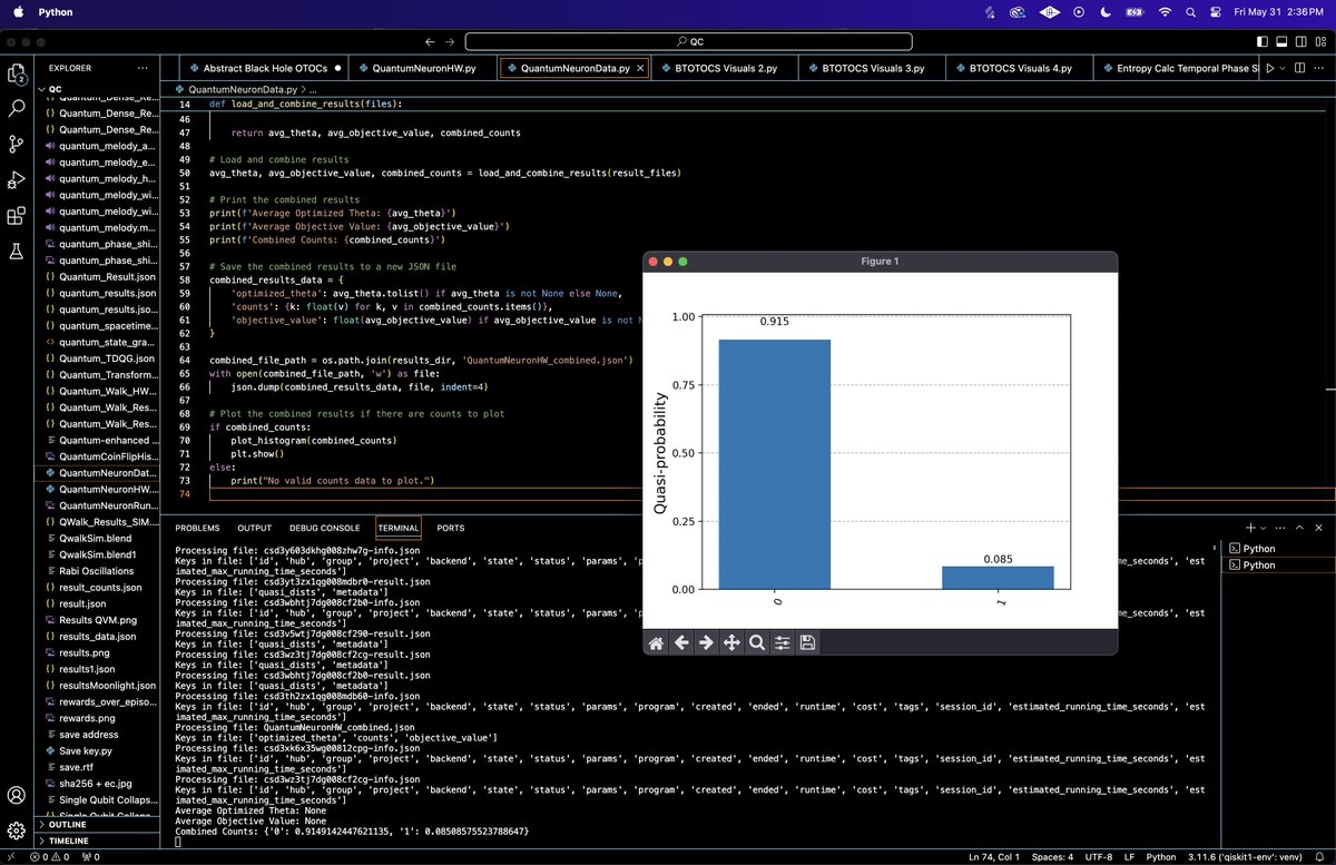
'0': 0.9149142447621135
'1': 0.08508575523788647
These combined counts represent the normalized measurement results from multiple runs of the quantum circuit.

Measurement Probabilities:
The probability of measuring the qubit in the '0' state is approximately 91.5%.
The probability of measuring the qubit in the '1' state is approximately 8.5%.

Quantum State and Expectation Values:
Given that we used a parameterized circuit involving a rotation around the z-axis and Hadamard gates, these probabilities indicate that the optimized parameter θ likely resulted in a state that is heavily biased towards the '0' state.
The expectation value of the Z observable can be computed as ⟨Z⟩ = P(0) − P(1), which in this case is 0.914914 − 0.085086 = 0.829828.

Optimization Insight:
The goal of our optimization was to find a parameter θ that minimizes the objective function, which was defined as (⟨Z⟩ − 1)^2. An expectation value of 0.829828 suggests that the objective function value is (0.829828 − 1)^2 = 0.02896.
This result indicates that our optimization process brought the expectation value close to 1, but not perfectly. The circuit parameter was likely near the optimal point but may not have fully converged within the allowed iterations.

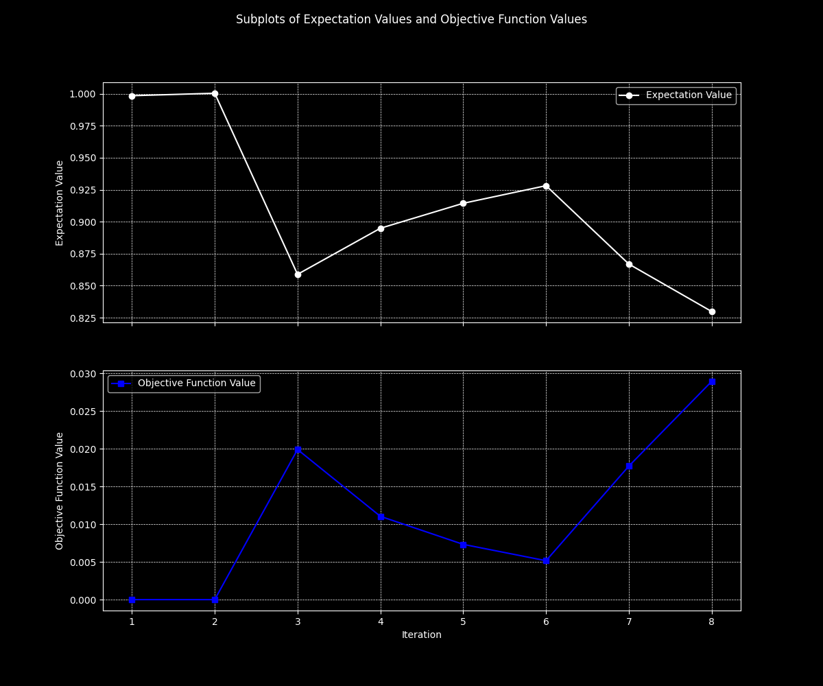
The subplots above illustrate the relationship between the expectation values and the objective function values over all iterations. On top, the Y-Axis is the expectation Value (⟨Z⟩) and X-Axis is Iteration. On bottom, the Y-Axis is objective Function Value and the X-Axis is iteration. The initial conditions were favorable, keeping the expectation value close to 1. The drop at the third iteration indicates a point where the optimization faced a challenge or required a parameter adjustment.
Effectiveness of the Quantum Gradient Descent: The fact that we reached an expectation value close to 1 suggests that the quantum gradient descent process was effective, though it could be improved with more iterations or more shots per iteration to reduce statistical noise. Given the constraints (e.g., limited iterations and shots), this result shows that the approach has potential but may require fine tuning for better accuracy. I will scale this with refreshed time next month.

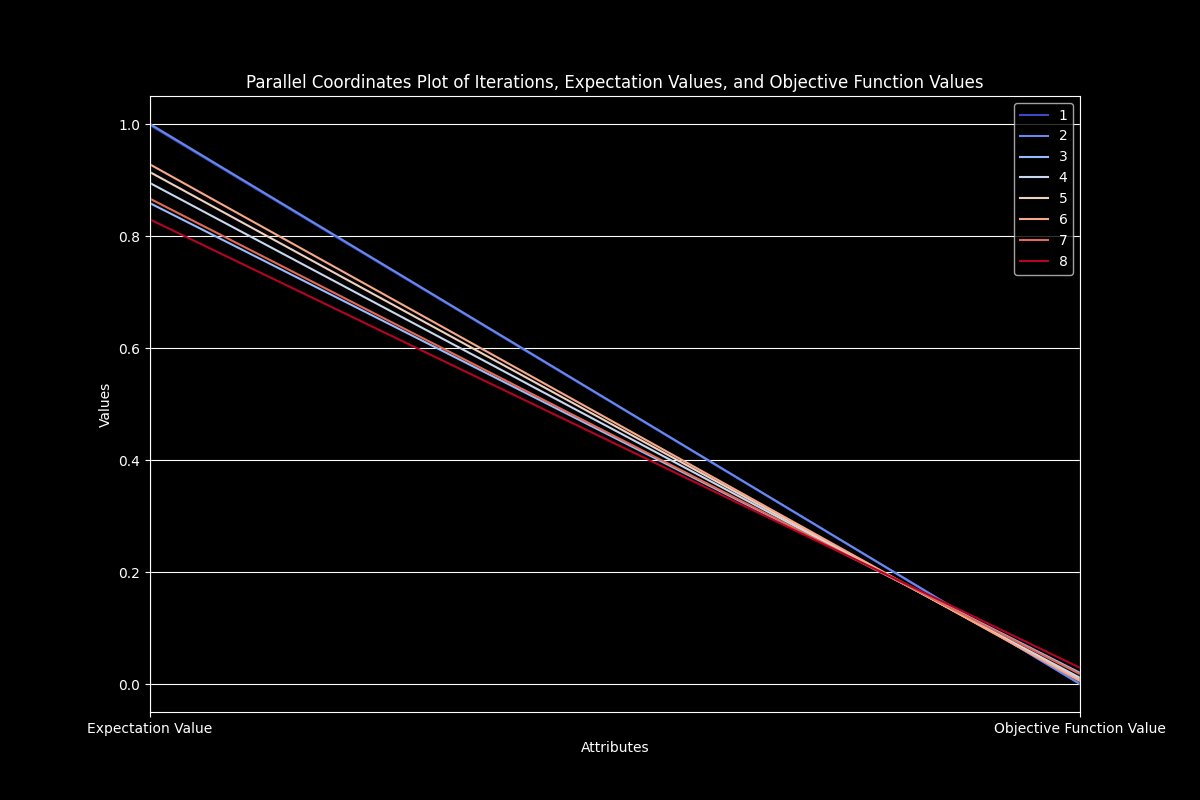
The Parallel Coordinates Plot above displays the relationship between iterations, expectation values, and objective function values. Each line represents an iteration and shows the corresponding expectation value and objective function value. The expectation value axis shows values close to 1 at the top. Most iterations start with high expectation values but vary as they move towards the objective function value axis. The objective function value axis shows values closer to 0 at the top. Lower objective function values indicate better optimization performance. Lines that remain close together suggest that the optimization process is converging. Lines that spread out indicate divergence or variability in the optimization performance.

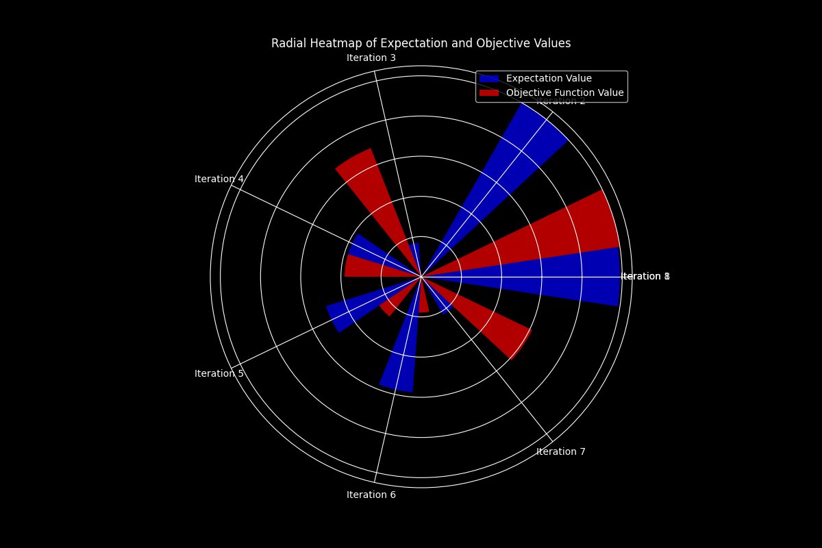
The Radial Heatmap above visualizes the distribution of expectation values and objective function values. Each segment (wedge) represents a different iteration. Blue segments represent expectation values and red segments represent objective function values. The radial length of each segment corresponds to the normalized values of expectation and objective function values. Large blue segments at iterations 3 and 6 indicate high expectation values, while small red segments at these points indicate low objective function values. Consistent performance can be seen where blue segments (expectation values) are close to the outer edge and red segments (objective function values) are near the center. Any deviation from this pattern indicates potential areas where the optimization faced challenges or noise affected performance.

Summary:
The combined measurement results from multiple runs of the experiment showed the following probabilities:
Measuring the qubit in the '0' state: 91.5%
Measuring the qubit in the '1' state: 8.5%
The expectation value of the Z observable, calculated as ⟨Z⟩ = P(0) − P(1), was found to be approximately 0.8298. The objective function value, (0.8298 − 1)^2, was approximately 0.0290. These results indicate that the optimization process was effective, bringing the expectation value close to the desired target of 1. However, the results suggest that further refinement, such as increasing the number of iterations or shots per iteration, could improve accuracy.
In the end, the experiment demonstrated the feasibility of implementing quantum gradient descent on IBM's quantum hardware.

Code:

# Imports
import numpy as np
from qiskit import QuantumCircuit, transpile
from qiskit_ibm_runtime import QiskitRuntimeService, Session, Sampler
from qiskit.circuit import Parameter
from scipy.optimize import minimize
import json
import logging

# Set up logging and IBM Quantum service
logging.basicConfig(level=logging.DEBUG, format='%(asctime)s - %(levelname)s - %(message)s')
API_KEY = 'Your_IBMQ_Key_O-`'  # Replace w/ IBMQ  key
service = QiskitRuntimeService(channel='ibm_quantum', token=API_KEY)
backend = service.backend('ibm_osaka')

# Define a parameterized quantum neuron circuit
theta = Parameter('θ')
qc = QuantumCircuit(1, 1)  # One qubit and one classical bit for output
qc.h(0)
qc.rz(theta, 0)
qc.h(0)
qc.measure(0, 0)

# Define the function to execute the circuit and retrieve the result
def execute_circuit(param_value):
    qc_temp = qc.assign_parameters({theta: param_value})
    transpiled_circuit = transpile(qc_temp, backend=backend, optimization_level=3)
    
    with Session(service=service, backend=backend) as session:
        sampler = Sampler()
        job = sampler. run(circuits=[transpiled_circuit], shots=512)
        result = job.result()
    
    counts = result.quasi_dists[0].binary_probabilities()
    return counts

# Compute the expectation value of the Z observable
def compute_expectation_value(counts):
    shots = sum(counts.values())
    expectation = (counts.get('0', 0) - counts.get('1', 0)) / shots
    return expectation

# Define the objective function for optimization
def objective_function(params):
    counts = execute_circuit(params[0])
    exp_val = compute_expectation_value(counts)
    return (exp_val - 1) ** 2

# Numerical gradient calculation using finite differences
def gradient_function(params):
    epsilon = 1e-6
    grad = np.zeros_like(params)
    for i in range(len(params)):
        params_eps = np.copy(params)
        params_eps[i] += epsilon
        grad[i] = (objective_function(params_eps) - objective_function(params)) / epsilon
    return grad

# Perform the backend runs and save each result to a separate JSON file
initial_point = np.array([0.0])
number_of_runs = 7  # Number of runs to perform

for run in range(1, number_of_runs + 1):
    # Perform gradient descent optimization
    result = minimize(objective_function, initial_point, jac=gradient_function, method='BFGS', options={'maxiter': 5})
    optimized_theta = result.x

    # Transpile and run the optimized circuit
    optimized_circuit = qc.assign_parameters({theta: optimized_theta[0]})
    transpiled_circuit = transpile(optimized_circuit, backend=backend, optimization_level=3)

    with Session(service=service, backend=backend) as session:
        sampler = Sampler()
        job = sampler. run(circuits=[transpiled_circuit], shots=512)
        result = job.result()

    # Analyze results
    counts = result.quasi_dists[0].binary_probabilities()
    logging. info(f"Counts from run {run}: {counts}")

    # Save results to JSON
    results_data = {
        'optimized_theta': optimized_theta.tolist(),
        'counts': {k: float(v) for k, v in counts.items()},
        'objective_value': float(objective_function(optimized_theta))
    }

    file_path = f'/Users/Documents/QuantumNeuronHW{run}.json'
    with open(file_path, 'w') as file:
        json.dump(results_data, file, indent=4)

Run Analysis Code: 
import json
import os
import numpy as np
from qiskit.visualization import plot_histogram
import matplotlib.pyplot as plt

# Directory containing the result files
results_dir = '/Users/Documents/QuantumNeuronRuns/'

# List all result files in the directory
result_files = [f for f in os.listdir(results_dir) if f.endswith('.json')]

# Function to load and combine results from JSON files
def load_and_combine_results(files):
    combined_counts = {}
    combined_theta = []  # Placeholder if we find optimized_theta in some files
    combined_objective_values = []  # Placeholder if we find objective_value in some files
    
    for file in files:
        with open(os.path.join(results_dir, file), 'r') as f:
            data = json.load(f)
            
            # Debugging: Print out the keys in each file
            print(f"Processing file: {file}")
            print(f"Keys in file: {list(data.keys())}")
            
            # Extract counts from quasi_dists
            if 'quasi_dists' in data:
                for dist in data['quasi_dists']:
                    for key, value in dist.items():
                        if key in combined_counts:
                            combined_counts[key] += value
                        else:
                            combined_counts[key] = value

    # Normalize combined counts
    total_counts = sum(combined_counts.values())
    if total_counts > 0:
        for key in combined_counts:
            combined_counts[key] /= total_counts
    
    # For the purpose of this task, optimized_theta and objective_value are not present
    # Return None for these values
    avg_theta = None
    avg_objective_value = None
    
    return avg_theta, avg_objective_value, combined_counts

# Load and combine results
avg_theta, avg_objective_value, combined_counts = load_and_combine_results(result_files)

# Print the combined results
print(f'Average Optimized Theta: {avg_theta}')
print(f'Average Objective Value: {avg_objective_value}')
print(f'Combined Counts: {combined_counts}')

# Save the combined results to a new JSON file
combined_results_data = {
    'optimized_theta': avg_theta.tolist() if avg_theta is not None else None,
    'counts': {k: float(v) for k, v in combined_counts.items()},
    'objective_value': float(avg_objective_value) if avg_objective_value is not None else None
}

combined_file_path = os.path.join(results_dir, 'QuantumNeuronHW_combined.json')
with open(combined_file_path, 'w') as file:
    json.dump(combined_results_data, file, indent=4)

# Plot the combined results if there are counts to plot
if combined_counts:
    plot_histogram(combined_counts)
    plt. show()
else:
    print("No valid counts data to plot.")
# end

Code to Analyze Runs (post hardware run):

import json
import os
import numpy as np
from qiskit.visualization import plot_histogram
import matplotlib.pyplot as plt

# Directory containing the result files
results_dir = '/Users/Documents/QuantumNeuronJobs/'

# List all result files in the directory
result_files = [f for f in os.listdir(results_dir) if f.endswith('.json')]

# Function to load and combine results from JSON files
def load_and_combine_results(files):
    combined_counts = {}
    expectation_values = []
    objective_values = []
    for file in files:
        with open(os.path.join(results_dir, file), 'r') as f:
            data = json.load(f)
            
            print(f"Processing file: {file}")
            print(f"Keys in file: {list(data.keys())}")
            
            if 'quasi_dists' in data:
                for dist in data['quasi_dists']:
                    for key, value in dist.items():
                        if key in combined_counts:
                            combined_counts[key] += value
                        else:
                            combined_counts[key] = value

                # Calculate expectation value
                P0 = combined_counts.get('0', 0)
                P1 = combined_counts.get('1', 0)
                total = P0 + P1
                if total > 0:
                    expectation_value = (P0 - P1) / total
                    expectation_values.append(expectation_value)
                    # Calculate objective value
                    objective_value = (expectation_value - 1) ** 2
                    objective_values.append(objective_value)

    # Normalize combined counts
    total_counts = sum(combined_counts.values())
    if total_counts > 0:
        for key in combined_counts:
            combined_counts[key] /= total_counts

    return expectation_values, objective_values, combined_counts

# Load and combine results
expectation_values, objective_values, combined_counts = load_and_combine_results(result_files)

# Print the combined results
print(f'Expectation Values: {expectation_values}')
print(f'Objective Values: {objective_values}')
print(f'Combined Counts: {combined_counts}')

# Save the combined results to a new JSON file
analysis_results = {
    'expectation_values': expectation_values,
    'objective_values': objective_values,
    'counts': {k: float(v) for k, v in combined_counts.items()}
}

analysis_file_path = '/Users/Documents/QNeuralAnalysis.json'
with open(analysis_file_path, 'w') as file:
    json.dump(analysis_results, file, indent=4)

# Plot the combined results
if combined_counts:
    plot_histogram(combined_counts)
    plt.title("Combined Measurement Outcomes")
    plt. show()

# Plot expectation values over iterations
if expectation_values:
    plt.plot(expectation_values, label='Expectation Value')
    plt.xlabel('Iteration')
    plt.ylabel('Expectation Value')
    plt.title('Expectation Value Over Iterations')
    plt.legend()
    plt. show()

# Plot objective values over iterations
if objective_values:
    plt.plot(objective_values, label='Objective Function Value')
    plt.xlabel('Iteration')
    plt.ylabel('Objective Function Value')
    plt.title('Objective Function Value Over Iterations')
    plt.legend()
    plt. show()
# end

Subplots of Expectation Values and Objective Function Values Code:

import json
import matplotlib.pyplot as plt
import numpy as np

# Load the analysis results
file_path = '/Users/Documents/QNeuralAnalysis.json'
with open(file_path, 'r') as file:
    data = json.load(file)

expectation_values = data['expectation_values']
objective_values = data['objective_values']
iterations = np.arange(1, len(expectation_values) + 1)

# Set plot style
plt. style.use('dark_background')

# Subplots of Expectation Values and Objective Function Values
fig, axs = plt.subplots(2, 1, figsize=(12, 10), sharex=True)
fig.suptitle('Subplots of Expectation Values and Objective Function Values', color='white')

axs[0].plot(iterations, expectation_values, 'o-', color='white', label='Expectation Value')
axs[0].set_ylabel('Expectation Value', color='white')
axs[0].grid(True, which='both', linestyle='--', linewidth=0.5)
axs[0].legend()

axs[1].plot(iterations, objective_values, 's-', color='blue', label='Objective Function Value')
axs[1].set_xlabel('Iteration', color='white')
axs[1].set_ylabel('Objective Function Value', color='white')
axs[1].grid(True, which='both', linestyle='--', linewidth=0.5)
axs[1].legend()

plt.savefig('/Users/Documents/Subplots_Expectation_Objective.png')
plt. show()
# end

Parallel Coordinates Plot Code:

import pandas as pd
import matplotlib.pyplot as plt
from pandas.plotting import parallel_coordinates

# Load the analysis results
file_path = '/Users/Documents/QNeuralAnalysis.json'
with open(file_path, 'r') as file:
    data = json.load(file)

expectation_values = data['expectation_values']
objective_values = data['objective_values']
iterations = np.arange(1, len(expectation_values) + 1)

# Create a DataFrame
df = pd.DataFrame({
    'Iteration': iterations,
    'Expectation Value': expectation_values,
    'Objective Function Value': objective_values
})

# Set plot style
plt. style.use('dark_background')

# Parallel Coordinates Plot
plt.figure(figsize=(12, 8))
parallel_coordinates(df, class_column='Iteration', colormap='coolwarm')
plt.title('Parallel Coordinates Plot of Iterations, Expectation Values, and Objective Function Values', color='white')
plt.xlabel('Attributes', color='white')
plt.ylabel('Values', color='white')
plt.savefig('/Users/Documents/Parallel_Coordinates.png')
plt. show()

Radial Heatmap Code:

import numpy as np
import matplotlib.pyplot as plt
from matplotlib.projections import PolarAxes
from matplotlib.spines import Spine
from matplotlib.projections.polar import PolarTransform
from matplotlib.ticker import FixedLocator

# Load the analysis results
file_path = '/Users/Documents/QNeuralAnalysis.json'
with open(file_path, 'r') as file:
    data = json.load(file)

expectation_values = data['expectation_values']
objective_values = data['objective_values']
iterations = np.arange(1, len(expectation_values) + 1)

# Normalize data for heatmap
normalized_expectation = (expectation_values - np.min(expectation_values)) / (np.max(expectation_values) - np.min(expectation_values))
normalized_objective = (objective_values - np.min(objective_values)) / (np.max(objective_values) - np.min(objective_values))

# Set plot style
plt. style.use('dark_background')

# Radial Heatmap
fig, ax = plt.subplots(figsize=(12, 8), subplot_kw=dict(polar=True))
theta = np.linspace(0, 2 * np.pi, len(iterations))

bars = ax. bar(theta, normalized_expectation, width=0.3, color='blue', alpha=0.7, label='Expectation Value')
bars = ax. bar(theta + 0.3, normalized_objective, width=0.3, color='red', alpha=0.7, label='Objective Function Value')

ax.set_xticks(theta)
ax.set_xticklabels([f'Iteration {i}' for i in iterations], color='white')
ax.set_yticklabels([])

ax.set_title('Radial Heatmap of Expectation and Objective Values', color='white')
ax.legend(loc='upper right')

plt.savefig('/Users/Documents/Radial_Heatmap.png')
plt. show()
# end.