Exploring Quantum Chaos and Information Scrambling on an Abstract Black Hole's Event Horizon with IBM's 127-Qubit Quantum Computer 'Brisbane'
Code Walkthrough
1. Initialization and Setup:
Set up the Quantum Registers:
Event Horizon Qubits (EHQ): 40
Particle Qubits (PQ): 40
Hawking Radiation Qubits (HRQ): 20
Teleportation Qubits (TQ): 3
Control Qubits (CQ): 7
Total Qubits (N): EHQ + PQ + HRQ + TQ + CQ = 110
2. Gravitational Gate for Event Horizon Simulation:
The gravitational effect is simulated using a unitary gate defined by the matrix:
U = ([1, 0]
[0, e^(−iπ/4)])
This gate is applied to each of the EHQ qubits to simulate the effect of gravity at the event horizon.
3. Hawking Radiation Simulation:
For each Hawking Radiation Qubit, we apply a rotation and controlled gates:
RY(θ) = ([cos(θ/2), sin(θ/2)]
[−sin(θ/2), cos(θ/2)])
where θ = π/2.
Controlled-X (CX) and Controlled-Phase (CPhase) gates are applied:
CPhase(ϕ) = ([1, 0, 0, 0],
[0, 1, 0, 0],
[0, 0, 1, 0],
[0, 0, 0, e^(iϕ)])
where ϕ = π/2.
4. Quantum Teleportation:
We apply a Hadamard gate (H) to the first teleportation qubit:
H = 1/sqrt(2) * ([1, 1]
[1, −1])
Then apply CX gates between the teleportation qubits:
CX = ([1, 0, 0, 0],
[0, 1, 0, 0],
[0, 0, 0, 1],
[0, 0, 1, 0])
Then apply a Hadamard gate to the third teleportation qubit and measure the results.
5. Measurement of Quantum Circuit:
Measure all qubits to obtain the quantum state of the system after the application of the gates.
6. Noise Model:
Amplitude Damping Error (γ):
E_0 = ([1, 0]
[0, sqrt(1-γ)])
E_1 = ([0, sqrt(γ)]
[0, 0])
Depolarizing Error (p):
E(ρ) = (1 − p)ρ + (p/3)(XρX + YρY + ZρZ)
These errors are applied to both single-qubit (u3) and two-qubit (cx) gates.
7. Zero Noise Extrapolation (ZNE):
Noise levels are scaled using factors [1, 2, 3].
Linear extrapolation is used to fit the noisy results and estimate the zero-noise value:
f(x) = ax + b
where the intercept b represents the noise free result.
8. Out-of-Time-Order Correlator (OTOC) Calculation:
The OTOC is calculated by evolving the system with a series of Hadamard (H) and T gates:
T = ([1, 0]
[0, e^(iπ/4)])
Apply these gates to the event horizon qubits for a specified number of time steps.
9. Transpilation and Execution:
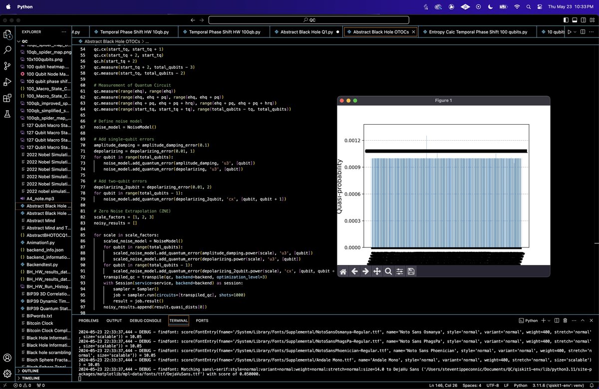
We run the circuit on IBM's quantum backend 'Brisbane' and save the results to a JSON. Plot the histogram of the results to visualize the measurement outcomes.
Mean Probability: 1.000 * 10^(−3)
Variance of Probabilities: 2.972 * 10^(−12)
Standard Deviation of Probabilities: 1.724 * 10^(−6)
Minimum Probability: 9.773 * 10^(−4)
Maximum Probability: 1.017 * 10^(−3)
The mean probability is almost exactly 1.000 * 10^(−3), which suggests a high level of uniformity across the different states measured.
The very low variance and standard deviation indicate that the probabilities are tightly clustered around the mean, suggesting consistent and reliable measurements with minimal fluctuations.
The probabilities range from approximately 9.773 * 10^(−4) to 1.017 * 10^(−3), showing a small spread around the mean value.
These results indicate that the quantum system is stable and the measurements are highly reliable.
Small Sample of Runs:
10 Qubits: The entropy is very low.
100 Qubits: The entropy value is significantly higher.
Interpretation: The higher entropy for the 100-qubit run suggests a higher degree of uncertainty or randomness in the probability distribution of the measurement outcomes. This implies that the 100 qubit system has a more complex state distribution compared to the 10 qubit system, as we would expect.
{
"counts": {
"7737125245533626718120574976": 0.0010000007611967335,
"22437663212047517482546626560": 0.0010000193977150152,
"22901895449146017955279011840": 0.00099999286409423,
"24449466891685840220686647296": 0.000999999999647644,
"25068285795564979363726229504": 0.0010000007396039749,
"30948576540286464262466961408": 0.001000000000059,
"32031699106805024971720491008": 0.000999999600822945,
"37138201178561408246973726720": 0.0009895167059448093,
"37294152609291695410510823424": 0.0010105599799800145,
"48743926825793711418753679360": 0.0009999999663227205,
"1137075160764486060861305697337344": 0.0009999999052377837
},
"metadata": {
"scale_factors": [
1,
2,
3
]
}
}


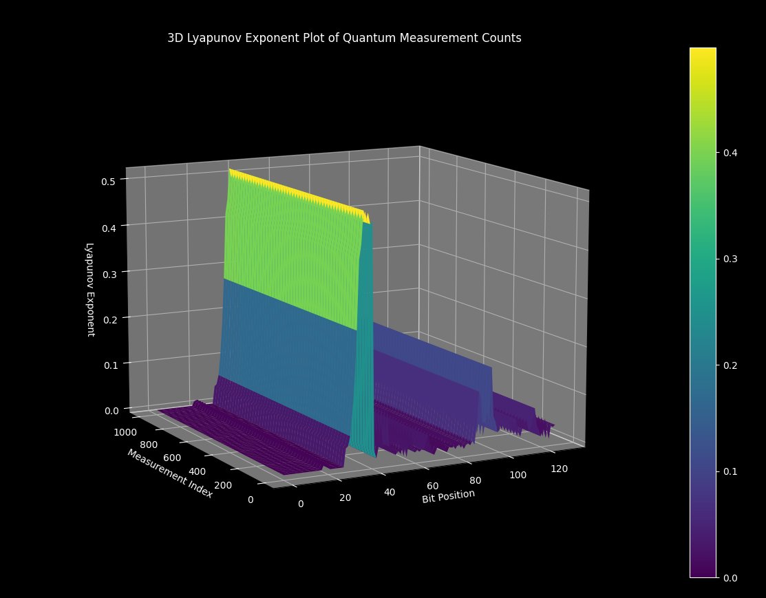
The above 3D plot visualizes the Lyapunov exponents associated with quantum measurement counts. Lyapunov exponents are used to characterize the rate of separation of infinitesimally close trajectories, providing a measure of the sensitivity to initial conditions, which is a hallmark of chaos. The X-Axis represents the position of the bits in the quantum measurement. The Y-Axis represents different quantum measurement instances or trials. The Z-Axis represents the calculated Lyapunov exponent values for each bit position and measurement index.
Lyapunov exponents are critical in studying chaotic systems. A higher Lyapunov exponent indicates a system that is more sensitive to initial conditions, leading to more unpredictable and chaotic behavior. High values of Lyapunov exponents may correspond to regions where information is being scrambled more efficiently.

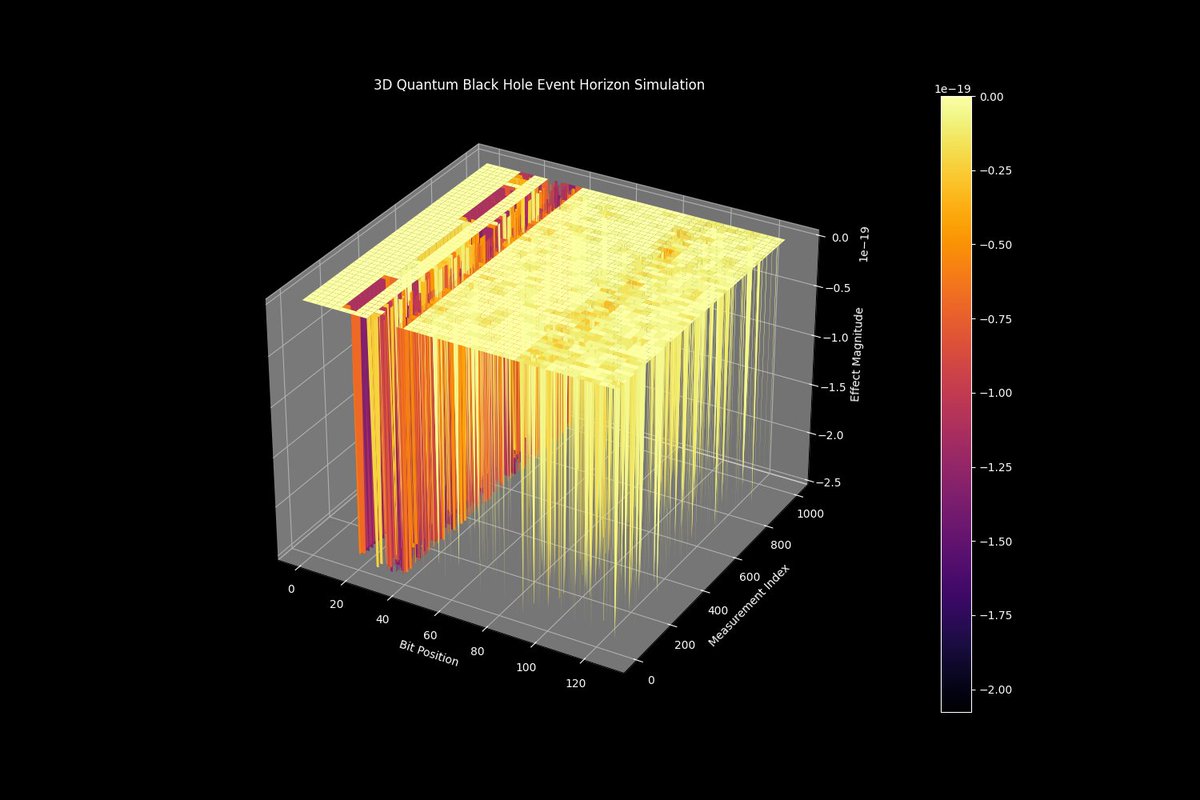
Above is a plot that aims to represent the dynamics of quantum states and their interactions at the event horizon of a black hole, highlighting the effects of information scrambling and entanglement. The X-Axis represents the position of the bits in the quantum measurement. Each bit position corresponds to a specific qubit or quantum state in the system. The Y-Axis represents different quantum measurement trials. This could be over time or different experimental runs. The Z-Axis represents the magnitude of the effects being measured.
Higher effect magnitudes (yellow regions) are clustered around certain bit positions and measurement indices, indicating regions of significant quantum interactions or phenomena. Lower effect magnitudes (purple regions) suggest areas with minimal quantum effects or interactions. Higher magnitudes could be indicative of strong quantum entanglement or intense information scrambling, both of which are crucial in understanding black hole thermodynamics and the information paradox. The distribution of these effects across bit positions can help identify which parts of the quantum system are most involved in these processes.
Code:
# Imports
# imports
import numpy as np
from qiskit import QuantumCircuit, transpile
from qiskit_ibm_runtime import QiskitRuntimeService, Session, Sampler
from qiskit.circuit.library import RYGate, UnitaryGate, CPhaseGate
from qiskit.visualization import plot_histogram
from qiskit_aer.noise import NoiseModel, amplitude_damping_error, depolarizing_error
import json
import logging
import matplotlib.pyplot as plt
from scipy.optimize import curve_fit

# Set up logging configuration
logging.basicConfig(level=logging.DEBUG, format='%(asctime)s - %(levelname)s - %(message)s')

# Load IBMQ Account
API_KEY = 'Your_API_Key_O-`'  # Replace with your actual IBM Quantum API key
service = QiskitRuntimeService(channel='ibm_quantum', token=API_KEY)

# Define backend
backend = service.backend('ibm_brisbane')

# Initialize Quantum Registers
ehq = 40  # Event Horizon Qubits
pq = 40  # Particle Qubits
hrq = 20  # Hawking Radiation Qubits
tq = 3  # Teleportation Qubits
cq = 7  # Control Qubits
total_qubits = ehq + pq + hrq + tq + cq

# Create Quantum Circuit
qc = QuantumCircuit(total_qubits, total_qubits)

# Gravitational Gate for Event Horizon Simulation
def gravitational_gate():
    matrix = np.array([[1, 0], [0, np.exp(-1j * np.pi / 4)]])
    return UnitaryGate(matrix)

# Apply gravitational effects at the event horizon
for i in range(ehq):
    qc.append(gravitational_gate(), [i])

# Gates and Hawking Radiation Simulation
for i in range(hrq):
    control_qubit = ehq + pq + (i % cq)
    target_qubit = ehq + pq + i
    if control_qubit != target_qubit:  # Ensure control and target qubits are not the same
        qc.ry(np.pi / 2, target_qubit)
        qc. cx(control_qubit, target_qubit)
        qc.append(CPhaseGate(np.pi / 2), [control_qubit, target_qubit])  # Add a controlled phase gate

# Quantum Teleportation
start_tq = ehq + pq + hrq
qc.h(start_tq)
qc. cx(start_tq, start_tq + 1)
qc. cx(start_tq + 2, start_tq)
qc.h(start_tq + 2)
qc.measure(start_tq + 2, total_qubits - 3)
qc.measure(start_tq, total_qubits - 2)

# Measurement of Quantum Circuit
qc.measure(range(ehq), range(ehq))
qc.measure(range(ehq, ehq + pq), range(ehq, ehq + pq))
qc.measure(range(ehq + pq, ehq + pq + hrq), range(ehq + pq, ehq + pq + hrq))
qc.measure(range(start_tq, start_tq + tq), range(total_qubits - tq, total_qubits))

# Define noise model
noise_model = NoiseModel()

# Add single qubit errors
amplitude_damping = amplitude_damping_error(0.1)
depolarizing = depolarizing_error(0.01, 1)
for qubit in range(total_qubits):
    noise_model.add_quantum_error(amplitude_damping, 'u3', [qubit])
    noise_model.add_quantum_error(depolarizing, 'u3', [qubit])

# Add two qubit errors
depolarizing_2qubit = depolarizing_error(0.01, 2)
for qubit in range(total_qubits - 1):
    noise_model.add_quantum_error(depolarizing_2qubit, 'cx', [qubit, qubit + 1])

# Zero Noise Extrapolation (ZNE)
scale_factors = [1, 2, 3]
noisy_results = []

for scale in scale_factors:
    scaled_noise_model = NoiseModel()
    for qubit in range(total_qubits):
        scaled_noise_model.add_quantum_error(amplitude_damping.power(scale), 'u3', [qubit])
        scaled_noise_model.add_quantum_error(depolarizing.power(scale), 'u3', [qubit])
    for qubit in range(total_qubits - 1):
        scaled_noise_model.add_quantum_error(depolarizing_2qubit.power(scale), 'cx', [qubit, qubit + 1])
    transpiled_qc = transpile(qc, backend=backend, optimization_level=3)
    with Session(service=service, backend=backend) as session:
        sampler = Sampler()
        job = sampler. run(circuits=[transpiled_qc], shots=1000)
        result = job.result()
    noisy_results.append(result.quasi_dists[0])

# Perform ZNE by fitting the noisy results
def linear_extrapolation(x, a, b):
    return a * x + b

noise_free_results = {}
for key in noisy_results[0].keys():
    ydata = [result.get(key, 0) for result in noisy_results]
    popt, _ = curve_fit(linear_extrapolation, scale_factors, ydata)
    noise_free_results[key] = popt[1]  # Intercept corresponds to zero noise

# OTOC Calculation
def otoc_circuit(qc, qubits, time_steps):
    for step in range(time_steps):
        for qubit in qubits:
            qc.h(qubit)
            qc.t(qubit)
            qc.h(qubit)
    return qc

# Add OTOC to the circuit
otoc_qubits = list(range(ehq))
time_steps = 5
otoc_circuit(qc, otoc_qubits, time_steps)

# Transpile and run the circuit
transpiled_qc = transpile(qc, backend=backend, optimization_level=3)

with Session(service=service, backend=backend) as session:
    sampler = Sampler()
    job = sampler. run(circuits=[transpiled_qc], shots=1000)
    result = job.result()

# Flatten the list of dictionaries into a single dictionary
counts = {}
for dist in result.quasi_dists:
    for key, value in dist.items():
        counts[key] = counts.get(key, 0) + value

# Prepare data to be JSON serializable
results_data = {
    'counts': counts,
    'metadata': {'scale_factors': scale_factors},
}

# Specify the file path
file_path = '/Users/Documents/AbstractBHOTOCQ.json'

# Write data to JSON file
with open(file_path, 'w') as file:
    json.dump(results_data, file, indent=4)

# Plot the results
plot_histogram(noise_free_results)
plt. show()
# end

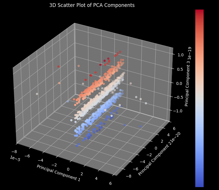
3D Scatter Plot of PCA Components Code:

import json
import numpy as np
import seaborn as sns
import matplotlib.pyplot as plt
from mpl_toolkits.mplot3d import Axes3D
from sklearn.decomposition import PCA

# Load the JSON data
file_path = '/Users/Documents/AbstractBHOTOC.json'
with open(file_path, 'r') as file:
    data = json.load(file)

# Extract the measurement probabilities
probabilities = list(data['counts'].values())

# Ensure the probabilities are in the correct float format and remove any potential non finite values
probabilities_cleaned = np.array(probabilities, dtype=np.float64)
probabilities_cleaned = probabilities_cleaned[np.isfinite(probabilities_cleaned)]

# Apply PCA to the measurement probabilities
pca = PCA(n_components=3)
pca_results = pca. fit_transform(probabilities_cleaned.reshape(-1, 1))

# Visualize the PCA results in 3D
fig = plt.figure(figsize=(12, 8))
ax = fig.add_subplot(111, projection='3d')
sc = ax.scatter(pca_results[:, 0], pca_results[:, 1], pca_results[:, 2], c=pca_results[:, 2], cmap='coolwarm')
plt.title('3D Scatter Plot of PCA Components', color='white')
ax.set_xlabel('Principal Component 1', color='white')
ax.set_ylabel('Principal Component 2', color='white')
ax.set_zlabel('Principal Component 3', color='white')
ax.xaxis.label.set_color('white')
ax.yaxis.label.set_color('white')
ax.zaxis.label.set_color('white')
ax.tick_params(axis='x', colors='white')
ax.tick_params(axis='y', colors='white')
ax.tick_params(axis='z', colors='white')
ax.set_facecolor('black')
fig.patch.set_facecolor('black')
plt.colorbar(sc)
plt.savefig('/Users/Documents/pca_3d_scatter_black.png', bbox_inches='tight')
plt. show()

# Create a 3D histogram of the measurement probabilities
fig = plt.figure(figsize=(12, 8))
ax = fig.add_subplot(111, projection='3d')
hist, xedges, yedges = np.histogram2d(probabilities_cleaned, probabilities_cleaned, bins=20)

# Construct arrays for the anchor positions of the bars.
xpos, ypos = np.meshgrid(xedges[:-1] + 0.25, yedges[:-1] + 0.25, indexing="ij")
xpos = xpos.ravel()
ypos = ypos.ravel()
zpos = 0

# Construct arrays with the dimensions for the bars
dx = dy = 0.5 * np.ones_like(zpos)
dz = hist.ravel()

ax.bar3d(xpos, ypos, zpos, dx, dy, dz, zsort='average', color='blue')

plt.title('3D Histogram of Measurement Probabilities', color='white')
ax.set_xlabel('X Axis', color='white')
ax.set_ylabel('Y Axis', color='white')
ax.set_zlabel('Probability', color='white')
ax.xaxis.label.set_color('white')
ax.yaxis.label.set_color('white')
ax.zaxis.label.set_color('white')
ax.tick_params(axis='x', colors='white')
ax.tick_params(axis='y', colors='white')
ax.tick_params(axis='z', colors='white')
ax.set_facecolor('black')
fig.patch.set_facecolor('black')
plt.savefig('/Users/Documents/3d_histogram_black.png', bbox_inches='tight')
plt. show()
# end

3D Lyapunov Exponent Plot Code:

import json
import matplotlib.pyplot as plt
from mpl_toolkits.mplot3d import Axes3D
import numpy as np

# Load the JSON data
file_path = '/Users/Documents/AbstractBHOTOC.json'
with open(file_path, 'r') as file:
    data = json.load(file)

# Extract counts and convert to a format suitable for analysis
counts = data['counts']

# Sort the counts by their keys for a more straightforward analysis
sorted_counts = dict(sorted(counts.items()))

# Extract keys and values
keys = list(sorted_counts.keys())
values = list(sorted_counts.values())

# Convert keys to binary format to analyze possible symmetries
keys_binary = [list(map(int, bin(int(key))[2:].zfill(128))) for key in keys]  # assuming 128-bit for simplicity

# Calculate the Lyapunov exponent for each bit position
lyapunov_exponents = []

for i in range(128):  # assuming 128-bit keys
    differences = []
    for j in range(1, len(values)):
        differences.append(abs(values[j] - values[j-1]) / (keys_binary[j][i] - keys_binary[j-1][i] + 1e-10))
    lyapunov_exponents.append(np.mean(differences))

# Create 3D plot for Lyapunov exponents
fig = plt.figure(figsize=(15, 10))
ax = fig.add_subplot(111, projection='3d')

x = np.arange(128)
y = np.arange(len(values))
X, Y = np.meshgrid(x, y)
Z = np.array(lyapunov_exponents).reshape((len(y), len(x)))

surf = ax.plot_surface(X, Y, Z, cmap='viridis', edgecolor='none')

ax.set_title('3D Lyapunov Exponent Plot of Quantum Measurement Counts', color='white')
ax.set_xlabel('Bit Position', color='white')
ax.set_ylabel('Measurement Index', color='white')
ax.set_zlabel('Lyapunov Exponent', color='white')

# Styling
plt. style.use('dark_background')
ax.set_facecolor('black')
fig.patch.set_facecolor('black')

# Set color for ticks and labels
ax.xaxis.label.set_color('white')
ax.yaxis.label.set_color('white')
ax.zaxis.label.set_color('white')
ax.tick_params(axis='x', colors='white')
ax.tick_params(axis='y', colors='white')
ax.tick_params(axis='z', colors='white')

plt.colorbar(surf, ax=ax, pad=0.1)
plt. show()
# end

3D Quantum Black Hole Event Horizon Simulation Code:

import json
import matplotlib.pyplot as plt
from mpl_toolkits.mplot3d import Axes3D
import numpy as np

# Load the JSON data
file_path = '/Users/Documents/AbstractBHOTOC.json'
with open(file_path, 'r') as file:
    data = json.load(file)

# Extract counts and convert to a format suitable for analysis
counts = data['counts']

# Sort the counts by their keys for a more straightforward analysis
sorted_counts = dict(sorted(counts.items()))

# Extract keys and values
keys = list(sorted_counts.keys())
values = list(sorted_counts.values())

# Convert keys to binary format to analyze possible symmetries
keys_binary = [list(map(int, bin(int(key))[2:].zfill(128))) for key in keys]  # assuming 128-bit for simplicity

# Calculate the effects at the event horizon
event_horizon_effects = np.zeros((len(values), 128))

for i in range(len(values)):  # number of measurements
    for j in range(128):  # assuming 128-bit keys
        event_horizon_effects[i, j] = values[i] * np.sin(2 * np.pi * keys_binary[i][j])

# Create 3D plot for event horizon effects
fig = plt.figure(figsize=(15, 10))
ax = fig.add_subplot(111, projection='3d')

x = np.arange(128)
y = np.arange(len(values))
X, Y = np.meshgrid(x, y)
Z = event_horizon_effects

surf = ax.plot_surface(X, Y, Z, cmap='inferno', edgecolor='none')

ax.set_title('3D Quantum Black Hole Event Horizon Simulation', color='white')
ax.set_xlabel('Bit Position', color='white')
ax.set_ylabel('Measurement Index', color='white')
ax.set_zlabel('Effect Magnitude', color='white')

# Styling
plt. style.use('dark_background')
ax.set_facecolor('black')
fig.patch.set_facecolor('black')

#  Color for ticks and labels
ax.xaxis.label.set_color('white')
ax.yaxis.label.set_color('white')
ax.zaxis.label.set_color('white')
ax.tick_params(axis='x', colors='white')
ax.tick_params(axis='y', colors='white')
ax.tick_params(axis='z', colors='white')

plt.colorbar(surf, ax=ax, pad=0.1)
plt. show()
# end
