Testing Entropy, Variance, and Standard Deviation between 10 and 100 Qubits on IBM's 127-Qubit Quantum Computer Sherbrooke

This experiment on IBM's 127-Qubit Quantum Computer 'Sherbrooke' uses superposition and interference within a system of qubits (w/ both 10 and 100 Qubit circuits), by utilizing a series of Hadamard and phase shift gates with qiskit. This experiment explores how quantum bits behave under sequential transformations, resulting in complex probability distributions observable after measurement. The goal is to analyze how entanglement and quantum coherence influence computational outcomes, and to compare entropy, variance, and standard deviation between a large and small set of Qubits.

Code Walkthrough

Step 1: Initialization:
The experiment begins with the initialization of a quantum circuit with x qubits. Initially, all qubits are in the ground state ∣0⟩.

Step 2: Superposition Creation:
A Hadamard gate (H-gate) is applied to each qubit. The H-gate transforms each qubit from the state ∣0⟩ to a superposed state:

H∣0⟩ = 1/sqrt(2) * (∣0⟩ + ∣1⟩)
This step places all qubits into a superposition of ∣0⟩ and ∣1⟩, creating a foundation for quantum interference.

Step 3: Phase Shift Application:
Over a series of time steps, a phase shift is introduced to each qubit. The phase shift for each qubit at a given time step t is calculated as:

θ(t) = (π/5)​ * t
The phase shift gate P(θ) is applied sequentially for each qubit according to the time step. The gate modifies the state of each qubit as follows:

P(θ)∣1⟩ = e^(iθ) * ∣1⟩
Thus, the state of each qubit after the phase shift is:

1/sqrt(2) * (∣0⟩ + e^(iθ) ∣1⟩)
This introduces relative phases between the states.

Step 4: Reapplication of Hadamard Gates:
After applying the phase shifts, a second round of Hadamard gates is applied to each qubit. The application of the H-gate again transforms each qubit's state. This step is crucial for recombining the probability amplitudes in a manner that reveals interference:

H(1/sqrt(2) * (∣0⟩ + e^(iθ) ∣1⟩)) = cos(θ/2) * ∣0⟩ + sin(θ/2) * ∣1⟩

Step 5: Measurement:
All qubits are then measured. The measurement collapses each qubit's wavefunction to either ∣0⟩ or ∣1⟩, with probabilities governed by their respective amplitudes. The outcome is a set of bit strings that represent the quantum state of each qubit.

Step 6: Data Analysis:
The resulting distribution of bit strings, or counts, is analyzed to determine the interference patterns. The counts are aggregated and visualized as a histogram, showing the probability distribution of obtaining each possible bit string from the quantum circuit.

Results:
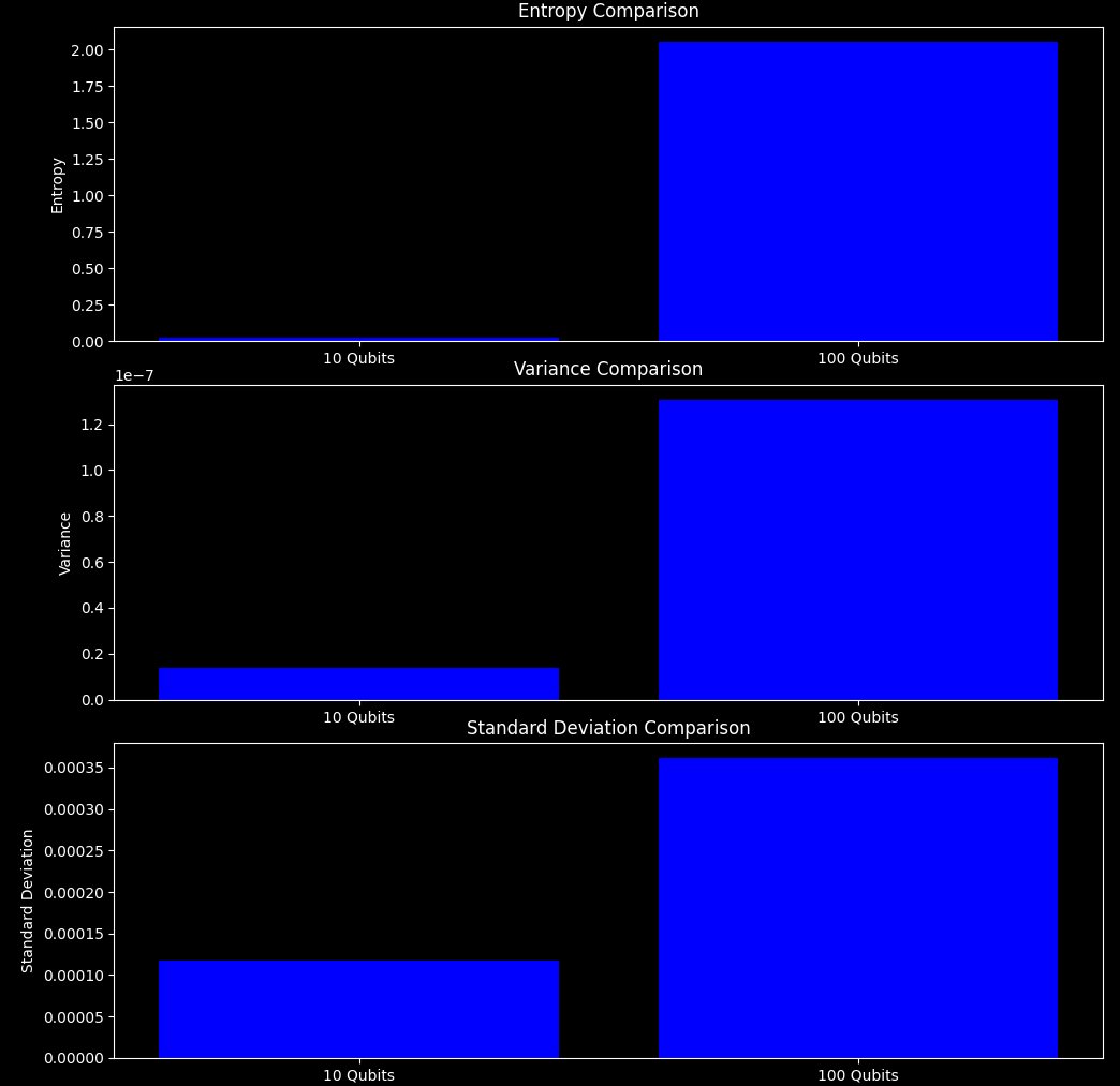
10 Qubits vs 100 Qubit Entropy, Variance, and Standard Deviation:

Entropy Comparison:
10 Qubits: The entropy is very low.
100 Qubits: The entropy value is significantly higher.
Interpretation: The higher entropy for the 100-qubit run suggests a higher degree of uncertainty or randomness in the probability distribution of the measurement outcomes. This implies that the 100 qubit system has a more complex state distribution compared to the 10 qubit system, as we would expect.

Variance Comparison:
10 Qubits: The variance is low, indicating that the measurement outcomes are tightly clustered around the mean.
100 Qubits: The variance is higher, indicating a wider spread of values in the measurement outcomes.
Interpretation: The higher variance for the 100-qubit system suggests greater variability in the outcomes. This is due to increased complexity and interactions among the qubits, leading to a more varied distribution of states.

Standard Deviation Comparison:
10 Qubits: The standard deviation is low, consistent with the low variance.
100 Qubits: The standard deviation is higher.
Interpretation: The higher standard deviation in the 100-qubit system further shows the increased spread of the data around the mean. This aligns with the observed higher variance and reflects the greater complexity of the system.
Thus, the increased entropy, variance, and standard deviation in the 100 qubit system indicate a more complex state. This complexity can be attributed to the increased number of qubits and their interactions, leading to a richer set of possible states and measurement outcomes.

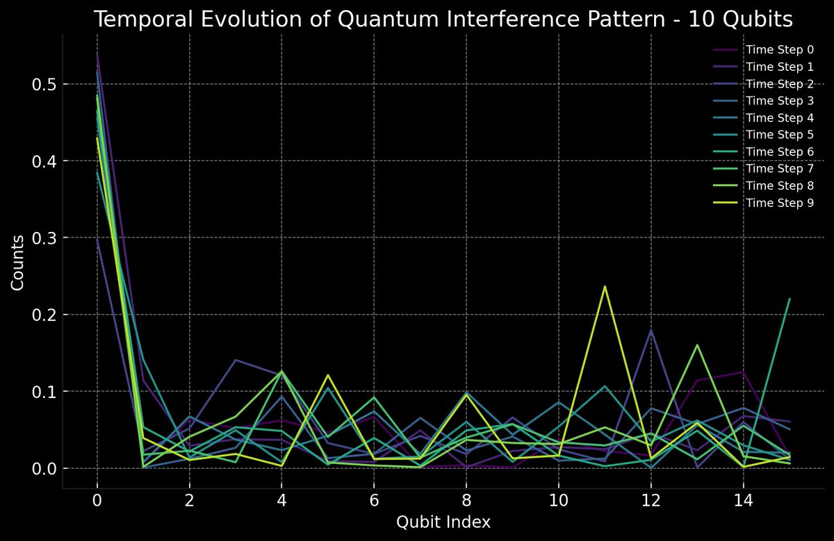
Temporal (phase) Evolution of Quantum Interference Pattern - 10 Qubits:

The 10-qubit chart shows the counts for each qubit index across 10 time steps (Time Step 0 to Time Step 9). The qubit index ranges from 0 to 14, indicating that the interference pattern is distributed across these indices. The counts are highest at Qubit Index 0 for all time steps, with the counts decreasing significantly for higher qubit indices.
The high counts at Qubit Index 0 suggest that the initial state of the system is highly likely to be in the ground state or low-index states. The variability and peaks at higher indices indicate that the quantum interference is causing the system to occasionally favor certain states over others.

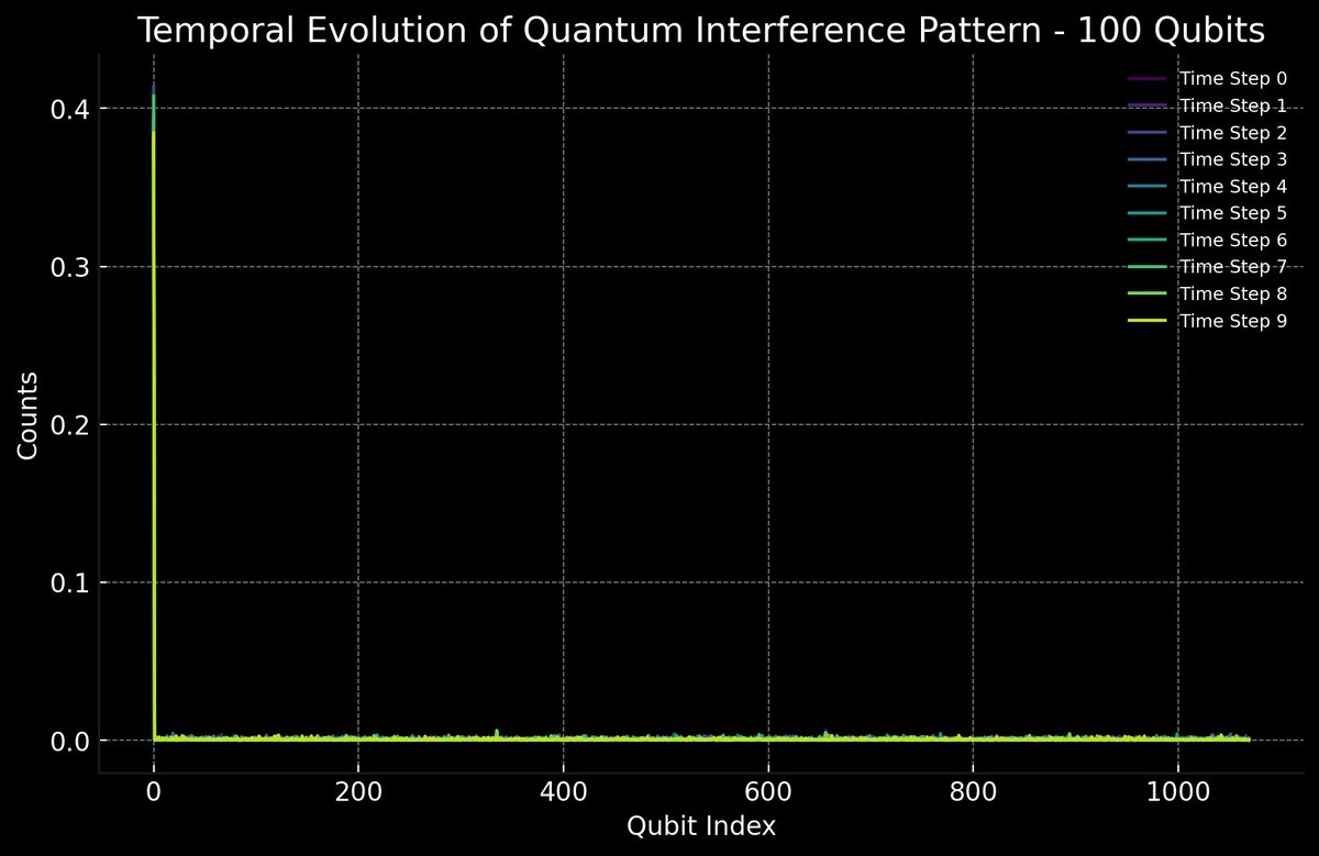
Temporal (phase) Evolution of Quantum Interference Pattern - 100 Qubits:

The 100-qubit chart also shows the counts for each qubit index across 10 time steps (Time Step 0 to Time Step 9). The lack of significant peaks and the very low counts at higher indices indicate that the 100-qubit system's interference pattern is more uniform and less variable compared to the 10-qubit system. The minimal changes over time suggest that the interference pattern for the 100-qubit system is more stable and less dynamic than the 10-qubit system.

Comparison:

Distribution:
The 10-qubit system shows more variability and noticeable peaks in its interference pattern, indicating more dynamic behavior and state transitions. The 100-qubit system has a more uniform distribution with less variability, suggesting a more stable and consistent interference pattern overall.

Time Evolution:
The 10-qubit system's interference pattern evolves more noticeably over time. The 100-qubit system shows minimal changes over time, indicating a more stable interference pattern.

Counts at Qubit Index 0:
Both systems have the highest counts at Qubit Index 0, indicating a high probability of the system being in the ground state or low-index states initially. The 10-qubit system has higher overall counts, while the 100-qubit system has much lower counts overall, reflecting the difference in system size and state distribution.
In the end, the temporal evolution of quantum interference patterns for both the 10-qubit and 100-qubit experiments highlights the differences in system behavior and stability. The 10-qubit system shows more dynamic and variable interference patterns, while the 100-qubit system exhibits a more stable and uniform pattern. These differences provide insights into how quantum systems scale and how interference patterns evolve with increasing qubit numbers, and how each may be used in different applications in qc.

Sample of Run Results:

10 Qubit Run:
{ "counts": { "0": 1.0455494082842536, "1": -0.000860880006311948, "2": -0.004970267586500554, "4": -0.030056775447914477, "6": 0.00037623114516605543, "8": -0.005541599576382072, "16": -0.0018882441063228204, "18": 0.00025904437070829473, "32": -0.00012584300903081363, "64": 0.0004997431971844846, "128": -0.0017669071342185346, "136": 0.000259208048016156, "256": -0.0030207206217459075, "288": 0.00024869105170483865, "320": 0.0002427589576944104, "512": 0.0007961524336992015 }, "metadata": [ { "shots": 4000, "circuit_metadata": {}, "readout_mitigation_overhead": 1.3551273269579631, "readout_mitigation_time": 0.09269230673089623 } ], "job_id": "cs1b7fnyhpyg008ah3wg" } Statistical Metrics (10 Qubits): Variance: 1.3712896312641474 * 10^(−8) Standard Deviation: 0.00011710207646596825 Entropy: 0.022529071985102518

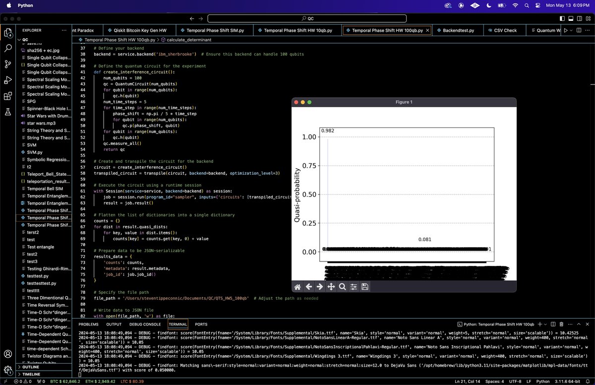
100 Qubit Run(sample):
{ "counts": { "0": 0.982280305592919, "1": -0.0008963588382386603, "2": -0.0015320938549815636, "4": 0.00018640172027664016, "8": -0.0015395188708829616, "16": -0.0005029830675843712, "32": 0.000622335300319988, "64": 0.0003029474283125386, "128": -0.0019328704189588918, "256": -0.0017285253331907416, "512": 0.0008267452211822403, "1024": -0.00040482944810949536, "2048": -0.0010897960965060042, "2176": 0.0002613161885392869, "4096": 0.0009803108221310638, ..., }, "metadata": [ { "shots": 4000, "circuit_metadata": {}, "readout_mitigation_overhead": 44.79382793591537, "readout_mitigation_time": 1.8307094699703157 } ], "job_id": "cs1bja14amg00087f6jg" }

Statistical Metrics (100 Qubits):
Variance: 1.3062278269064 * 10^(−7) Standard Deviation: 0.0003614177398670962 Entropy: 2.0551948622801746

Code:

# Imports
import numpy as np
from qiskit import QuantumCircuit, transpile
from qiskit_ibm_runtime import QiskitRuntimeService, Session
from qiskit.visualization import plot_histogram
import json
import logging
import matplotlib.pyplot as plt

# Set up logging configuration
logging.basicConfig(level=logging.DEBUG, format='%(asctime)s - %(levelname)s - %(message)s')

def calculate_determinant(matrix):
    logging.debug("Calculating determinant of the matrix: %s", matrix)
    try:
        # Check if the matrix is singular using the condition number
        cond_number = np.linalg.cond(matrix)
        if cond_number < 1 / np.finfo(matrix.dtype).eps:
            logging.debug("Matrix is well-conditioned.")
            return np.linalg.det(matrix)
        else:
            logging.warning("Matrix is poorly conditioned or singular. Condition number: %s", cond_number)
            # Adding a small identity matrix             regularization = 1e-10
            regularized_matrix = matrix + np.eye(matrix.shape[0]) * regularization
            det = np.linalg.det(regularized_matrix)
            logging.debug("Determinant after regularization: %s", det)
            return det
    except np.linalg.LinAlgError as e:
        logging.error("Error in determinant calculation: %s", e)
        return None

# Initialize Qiskit runtime service with IBMQ key
API_KEY = 'Your_IBMQ_Key_O-`'  
service = QiskitRuntimeService(channel='ibm_quantum', token=API_KEY)

# Define  backend
backend = service.backend('ibm_sherbrooke')

# Define the quantum circuit 
def create_interference_circuit():
    qc = QuantumCircuit(10)
    num_qubits = 10
    for qubit in range(num_qubits):
        qc.h(qubit)
    num_time_steps = 5
    for time_step in range(num_time_steps):
        phase_shift = np.pi / 5 * time_step
        for qubit in range(num_qubits):
            qc.p(phase_shift, qubit)
    for qubit in range(num_qubits):
        qc.h(qubit)
    qc.measure_all()
    return qc

# Create and transpile the circuit for the backend
circuit = create_interference_circuit()
transpiled_circuit = transpile(circuit, backend=backend, optimization_level=3)

# Execute the circuit using a runtime session
with Session(service=service, backend=backend) as session:
    job = session. run(program_id="sampler", inputs={'circuits': [transpiled_circuit]})
    result = job.result()

# Flatten the list of dictionaries into a single dictionary
counts = {}
for dist in result.quasi_dists:
    for key, value in dist.items():
        counts[key] = counts.get(key, 0) + value

# Prepare data to be JSON serializable
results_data = {
    'counts': counts,
    'metadata': result.metadata,
    'job_id': job.job_id()
}

# Path
file_path = '/Users/Documents/QTS_HW_10qb.json'

# Write data to JSON file
with open(file_path, 'w') as file:
    json.dump(results_data, file, indent=4)

# Plot the results
plot_histogram(counts)
plt. show()
# end

(100 Qubit Circuit)
# Imports
import numpy as np
from qiskit import QuantumCircuit, transpile
from qiskit_ibm_runtime import QiskitRuntimeService, Session
from qiskit.visualization import plot_histogram
import json
import logging
import matplotlib.pyplot as plt

# Set up logging configuration
logging.basicConfig(level=logging.DEBUG, format='%(asctime)s - %(levelname)s - %(message)s')

def calculate_determinant(matrix):
    logging.debug("Calculating determinant of the matrix: %s", matrix)
    try:
        # Check if the matrix is singular using the condition number
        cond_number = np.linalg.cond(matrix)
        if cond_number < 1 / np.finfo(matrix.dtype).eps:
            logging.debug("Matrix is well-conditioned.")
            return np.linalg.det(matrix)
        else:
            logging.warning("Matrix is poorly conditioned or singular. Condition number: %s", cond_number)
            # Adding a small identity matrix 
            regularization = 1e-10
            regularized_matrix = matrix + np.eye(matrix.shape[0]) * regularization
            det = np.linalg.det(regularized_matrix)
            logging.debug("Determinant after regularization: %s", det)
            return det
    except np.linalg.LinAlgError as e:
        logging.error("Error in determinant calculation: %s", e)
        return None

# Initialize Qiskit runtime service with IBMQ API key
API_KEY = 'Your_IBMQ_Key_O-`'  
service = QiskitRuntimeService(channel='ibm_quantum', token=API_KEY)

# Define backend
backend = service.backend('ibm_sherbrooke')  # Ensure this backend can handle 100 qubits

# Define the quantum circuit
def create_interference_circuit():
    num_qubits = 100
    qc = QuantumCircuit(num_qubits)
    for qubit in range(num_qubits):
        qc.h(qubit)
    num_time_steps = 5
    for time_step in range(num_time_steps):
        phase_shift = np.pi / 5 * time_step
        for qubit in range(num_qubits):
            qc.p(phase_shift, qubit)
    for qubit in range(num_qubits):
        qc.h(qubit)
    qc.measure_all()
    return qc

# Create and transpile the circuit for the backend
circuit = create_interference_circuit()
transpiled_circuit = transpile(circuit, backend=backend, optimization_level=3)

# Execute the circuit using a runtime session
with Session(service=service, backend=backend) as session:
    job = session. run(program_id="sampler", inputs={'circuits': [transpiled_circuit]})
    result = job.result()

# Flatten the list of dictionaries into a single dictionary
counts = {}
for dist in result.quasi_dists:
    for key, value in dist.items():
        counts[key] = counts.get(key, 0) + value

# Prepare data to be JSON serializable
results_data = {
    'counts': counts,
    'metadata': result.metadata,
    'job_id': job.job_id()
}

# File path
file_path = '/Users/Documents/QTS_HW_100qb'  

# Write data to JSON file
with open(file_path, 'w') as file:
    json.dump(results_data, file, indent=4)

# Plot the results
plot_histogram(counts)
plt. show()
# end