Exploring abstract Electron-Positron Annihilation on IBM's 127-Qubit Quantum Computer Osaka
Leveraging quantum computing and Qiskit, particle interactions can be abstractly represented and studied, offering a novel way for exploring complex probabilistic phenomena in particle physics. Quantum computers harness superposition and entanglement properties of quantum bits (qubits) to simulate the dynamics of particle interactions more efficiently than classical computers. By encoding the states and interactions of particles into quantum circuits, we can simulate various scattering processes, decay channels, and particle production mechanisms. Quantum computers could enable the exploration quantum tunneling effects, strong and weak force interactions, and the behavior of particles in extreme conditions such as those encountered in high energy collisions.
This experiment explores the abstract annihilation process of an electron-positron pair through quantum computing. Electrons and positrons, fundamental particles with opposite charges and identical masses, exhibit unique interactions when brought together. Upon collision, they can annihilate each other, leading to the creation of various particles, such as photons, neutrinos, or muons. This experiment aims to abstractly create the beginning of this process using a quantum circuit.
Code Walkthrough
1. Initialization:
We define a quantum circuit with two qubits, symbolizing the electron and positron states.
Applying Hadamard gates (H) to both qubits, we establish superposition states, ensuring they exist in a coherent mixture of |0⟩ and |1⟩. The superposition state can be represented by the equation:
Applying this to both qubits, the initial state of the system is:
2. Annihilation Gate:
We define a bespoke gate, the annihilation gate, designed to emulate the interaction between the electron and positron. The annihilation process is simulated by a custom gate sequence that includes a controlled-NOT (CNOT) gate, a Hadamard gate, a Pauli-X gate, and another CNOT gate. This sequence is designed to reflect the transformation of the electron-positron pair into another state, mimicking the annihilation process. The CNOT gate entangles the qubits, reflecting the interaction between the electron and positron.
The annihilation gate comprises a sequence of quantum operations:
Implement a controlled-NOT (CNOT) gate, where the electron qubit serves as the control and the positron qubit as the target. Mathematically, this gate can be represented as:
Apply a Hadamard gate to the electron qubit to generate entanglement between the qubits. Mathematically, the Hadamard gate is represented as:
Employ a Pauli-X gate (or NOT gate) to flip the state of the electron qubit from |0⟩ to |1⟩. Apply another CNOT gate, this time with the positron qubit as the control and the electron qubit as the target.
3. Measurement:
Conduct measurements on both qubits to get the final outcome of the annihilation process. The act of measurement collapses the quantum superposition into definitive classical states.
4. Data Analysis:
Measurement counts, transpiled circuit, backend information, job ID, and execution status are saved to a JSON. We also generate a histogram of the frequency of different outcomes for the annihilation process.
Using backend: ibm_kyoto
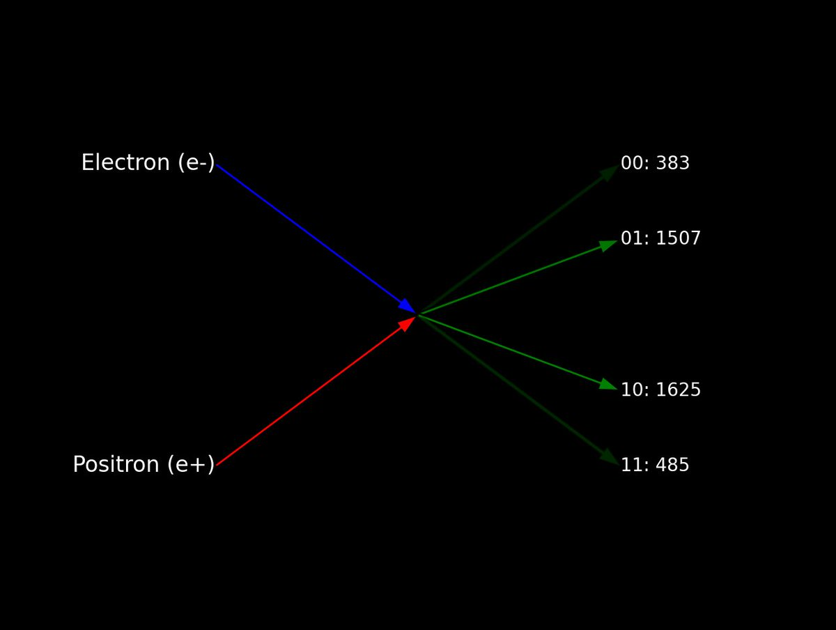
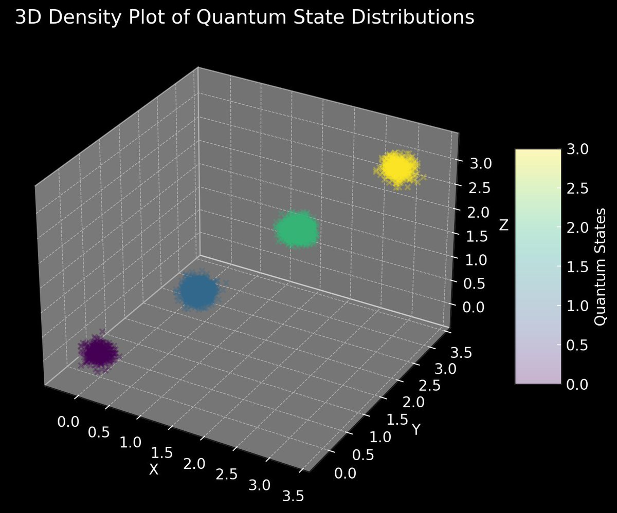
{'10': 1625, '11': 485, '00': 383, '01': 1507}
Probability of '00': 9.575%
Probability of '01': 37.675%
Probability of '10': 40.625%
Probability of '11': 12.125%

Probabilistic Nature vs. Deterministic Outcomes: While the quantum simulation inherently exhibits a probabilistic nature due to measurement, real-world annihilation events under specific conditions can have deterministic outcomes (e.g. exactly two photons produced). The quantum simulation mirrors the underlying quantum mechanics governing these processes, emphasizing the role of probability amplitudes and non-determinism. The higher probabilities for '01' and '10' can be abstractly interpreted as the simulation's equivalent of the conservation laws in real collisions, indicating a balance between the possible states post annihilation.
Symmetry and Quantum States: The simulation outcomes show a notable symmetry in probabilities, with '01' and '10' being more probable than '00' and '11'. This reflects the superposition and entanglement of quantum states where certain states are more likely due to the quantum gates applied, resembling the balanced outcomes expected in particle annihilation where different states (photon directions, polarizations) are equally probable in a symmetric setup.
Quantum Interference: The variation in probabilities can also be attributed to quantum interference effects, where the amplitude for certain outcomes constructively or destructively interferes. This is akin to the way probabilities for different quantum paths contribute to the observed outcomes in physical processes.


In the end, the simulation offers an abstract representation of an electron-positron annihilation. The higher probabilities for '01' and '10' could be abstractly interpreted as the simulation's equivalent of the conservation laws in real collisions, indicating a balance between the possible states post annihilation.
This type of quantum computation, in more complex ways, could serve as a bridge between abstract quantum theory and tangible experimental phenomena. Illustrating probabilistic principles of quantum mechanics and their possible implications for understanding the probabilities of particle interactions.
Code:
# imports
from qiskit import QuantumCircuit, Aer, transpile, IBMQ, execute
from qiskit.visualization import plot_histogram
import json
from datetime import datetime
import matplotlib.pyplot as plt
# IBM Quantum api and backend
IBMQ. save_account('Your_IBM_Key_O-', overwrite=True)
IBMQ.load_account()
provider = IBMQ.get_provider(hub='ibm-q')
backend = provider.get_backend('ibm_kyoto') # Adjust to your specific backend
print("Using backend: ", backend. name())
# Gate for annihilation process
def annihilation_gate(qc, electron_qubit, positron_qubit):
qc. cx(electron_qubit, positron_qubit)
qc.h(electron_qubit)
qc.x(electron_qubit)
qc. cx(positron_qubit, electron_qubit)
# Initialize a Quantum Circuit with 2 qubits (representing electron and positron)
qc = QuantumCircuit(2)
# Apply gates to represent the initial states of the electron and positron
qc.h(0)
qc.h(1)
# Apply custom annihilation gate
annihilation_gate(qc, 0, 1)
# Measure the qubits to observe the outcome
qc.measure_all()
# Transpile the circuit for the ibm_kyoto
transpiled_qc = transpile(qc, backend)
# Execute the circuit on the ibm_kyoto
job = execute(transpiled_qc, backend)
result = job.result()
counts = result.get_counts(transpiled_qc)
print(counts)
# Save relevant data to a JSON file
data = {
'measurement_counts': counts,
'circuit_transpiled': transpiled_qc.qasm(),
'backend': backend. name(),
'backend_properties': backend. properties().to_dict(),
'job_id': job.job_id(),
'status': job.status(),
'result_data': result. to_dict(),
'execution_date': datetime. now().strftime("%Y-%m-%d %H:%M:%S")
}
output_file = '/Users/Documents/ElectronPositronAnnihilation.json'
with open(output_file, 'w') as f:
json.dump(data, f, indent=4, default=str)
# Display histogram of measurement results with counts
plot_histogram(counts, title='Measurement Results', bar_labels=True)
plt. show()
# Feynman-like Diagram from Run Result Code
# imports
import json
import matplotlib.pyplot as plt
import numpy as np
# Load measurement counts from JSON
with open('/Users/Documents/ElectronPositronAnnihilation.json', 'r') as file:
measurement_counts = json.load(file)
# Define the figure for the Feynman-like diagram
fig, ax = plt.subplots(figsize=(8, 6))
ax.axis('off') # Remove the axis as they are not needed
ax.set_xlim([0, 4])
ax.set_ylim([0, 4])
# Define positions for the particles and vertices in the diagram
electron_position = (1, 3)
positron_position = (1, 1)
interaction_vertex = (2, 2)
outcomes_positions = {
'00': (3, 3),
'01': (3, 2.5),
'10': (3, 1.5),
'11': (3, 1)
}
# Draw electron and positron lines to the interaction vertex
ax.annotate('', xy=interaction_vertex, xytext=electron_position,
arrowprops=dict(facecolor='blue', shrink=0, width=2, headwidth=8))
ax.annotate('', xy=interaction_vertex, xytext=positron_position,
arrowprops=dict(facecolor='red', shrink=0, width=2, headwidth=8))
# Label the electron and positron
ax.text(*electron_position, 'Electron (e-)', ha='right', va='center', fontsize=12, color='white')
ax.text(*positron_position, 'Positron (e+)', ha='right', va='center', fontsize=12, color='white')
# Draw outcome lines and label them, using the counts as probability amplitudes
for state, position in outcomes_positions.items():
opacity = measurement_counts[state] / max(measurement_counts.values()) # Opacity based on relative count
ax.annotate('', xy=position, xytext=interaction_vertex,
arrowprops=dict(facecolor='green', alpha=opacity, shrink=0, width=2, headwidth=8))
ax.text(*position, f'{state}: {measurement_counts[state]}', ha='left', va='center', fontsize=10, color='white')
# bg color
fig.patch.set_facecolor('black')
ax.set_facecolor('black')
# Display the Feynman-like diagram
plt. show()