Quantum Cats: Encoding a Cat in 100 Quantum States
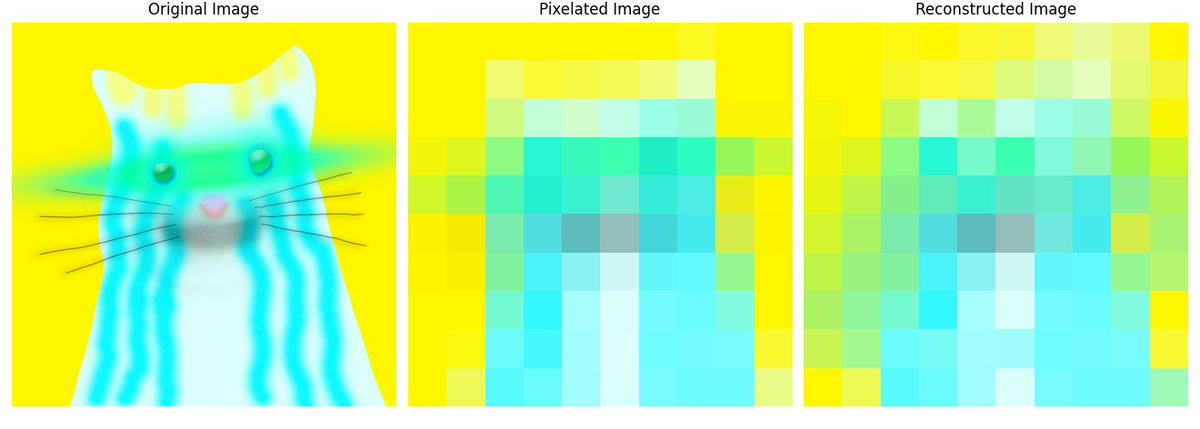
The experiment, using IBM's 127-qubit quantum computer Osaka and Qiskit, mixes quantum computing with image processing to place a Quantum Cat, in a Quantum Computer, for a brief second. The code encodes the cats color information into Qubits by using a series of quantum gates to represent RGB values, then retrieves the encoded data and recreates the quantum cat. the process showcases how quantum mechanics can potentially enhance or provide alternative methods for visual data encoding and retrieval. The end goal is to reconstruct the cats average colors from the quantum-encoded data, assessing the fidelity, and analyzing the effects of quantum noise and decoherence. Permanently putting this Quantum Cat into a Quantum Computers entropy, forever, for a second.
Code Walkthrough
1. Image Preparation:
A digital image is uploaded. This image is broken up into a matrix I of pixels, where each pixel p_(ij) has RGB components (R_(ij) ,G_(ij), B_(ij)).
2. Color Data Extraction:
The image I is resized for simplicity, maintaining aspect ratio when necessary, to reduce computational requirements and to adhere to our 127-qubit limit.
The image is then divided into ten horizontal segments, and for each segment S_k, the average color C_k = (R_k, G_k, B_k) is calculated by averaging the RGB values of all pixels within that segment.
3. Quantum State Preparation:
The average RGB values are normalized to a [0, 1] range via C_(norm) = Ck/255.
For each color component, a quantum state vector is prepared using rotation gates:
Red intensity is encoded using R_x(θ_r) where θ_r = 2π⋅R_(norm).
Green intensity is encoded using R_y(θ_g) where θ_g = 2π⋅G_(norm).
Blue intensity is encoded using R_z(θ_b) where θ_b = 2π⋅B_(norm).
The quantum state vector ∣ψ⟩ for each segment is the result of these rotations applied to the initial state ∣000⟩.
4. Quantum Circuit Execution:
A dynamical decoupling sequence is introduced to counteract decoherence. This is a series of X gates applied at specific intervals, effectively flipping the qubits and refocusing their phase evolution.
The state ∣ψ⟩ is then measured. If the measurement projective operator is M, the measurement result m_k for segment k is m_k = ⟨ψk∣ M ∣ψk⟩.
5. Measurement and Error Mitigation:
Calibration circuits are used to characterize the quantum computer's error profile. The Complete Measurement Fitter technique is applied to create a filter that mitigates these errors post-measurement.
6. Image Reconstruction:
The reconstructed image I is formed by assigning to each segment S_k a color based on the measurement outcome m_k.
If m_k corresponds to 111, the segment is colored with C_k; otherwise, it is set to black.
7. Result Visualization and Analysis:
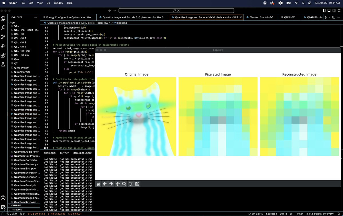
The original, average color, and reconstructed images are visualized to assess the quality of reconstruction and the effects of quantum errors.
8. Data:
The averaged color values and the quantum cats measurement results are serialized into a JSON format for documentation and further analysis.

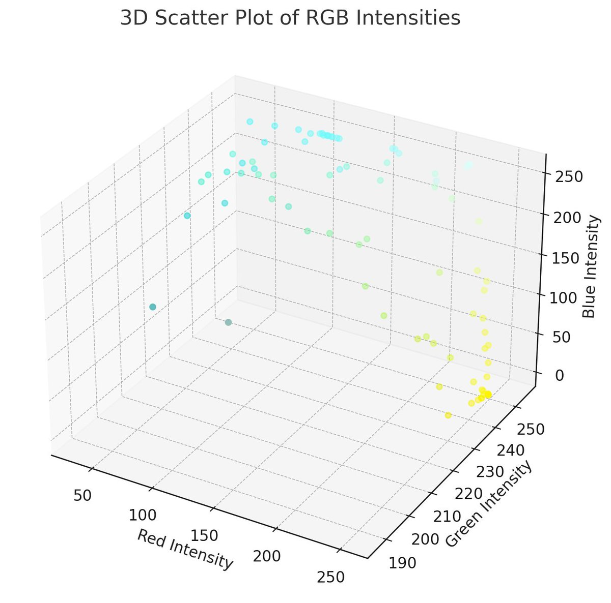
RGB color values and corresponding binary results for each of the 100 blocks in the 10x10 grid:
Block 1: RGB [255, 246, 0] - Binary Result: 1
Block 2: RGB [255, 246, 0] - Binary Result: 1
Block 3: RGB [255, 246, 0] - Binary Result: 0
Block 4: RGB [255, 246, 0] - Binary Result: 1
Block 5: RGB [255, 246, 0] - Binary Result: 0
Block 6: RGB [255, 246, 0] - Binary Result: 0
Block 7: RGB [255, 246, 1] - Binary Result: 0
Block 8: RGB [251, 248, 34] - Binary Result: 0
Block 9: RGB [255, 246, 0] - Binary Result: 0
Block 10: RGB [255, 246, 0] - Binary Result: 1
Block 11: RGB [255, 246, 0] - Binary Result: 0
Block 12: RGB [255, 246, 0] - Binary Result: 0
Block 13: RGB [241, 251, 114] - Binary Result: 0
Block 14: RGB [249, 249, 53] - Binary Result: 1
Block 15: RGB [246, 249, 68] - Binary Result: 1
Block 16: RGB [244, 249, 85] - Binary Result: 0
Block 17: RGB [241, 252, 123] - Binary Result: 0
Block 18: RGB [230, 254, 188] - Binary Result: 1
Block 19: RGB [255, 246, 0] - Binary Result: 0
Block 20: RGB [255, 246, 0] - Binary Result: 0
Block 21: RGB [255, 246, 0] - Binary Result: 0
Block 22: RGB [255, 246, 0] - Binary Result: 1
Block 23: RGB [208, 249, 127] - Binary Result: 0
Block 24: RGB [194, 254, 216] - Binary Result: 1
Block 25: RGB [208, 254, 207] - Binary Result: 0
Block 26: RGB [194, 254, 232] - Binary Result: 1
Block 27: RGB [155, 254, 230] - Binary Result: 1
Block 28: RGB [155, 251, 215] - Binary Result: 1
Block 29: RGB [250, 246, 4] - Binary Result: 0
Block 30: RGB [251, 246, 3] - Binary Result: 1
Block 31: RGB [243, 246, 11] - Binary Result: 0
Block 32: RGB [222, 247, 30] - Binary Result: 1
Block 33: RGB [140, 250, 131] - Binary Result: 1
Block 34: RGB [39, 247, 211] - Binary Result: 1
Block 35: RGB [57, 249, 188] - Binary Result: 0
Block 36: RGB [60, 254, 177] - Binary Result: 1
Block 37: RGB [32, 237, 196] - Binary Result: 0
Block 38: RGB [46, 252, 193] - Binary Result: 0
Block 39: RGB [151, 247, 90] - Binary Result: 1
Block 40: RGB [202, 247, 48] - Binary Result: 1
Block 41: RGB [208, 247, 42] - Binary Result: 0
Block 42: RGB [172, 244, 69] - Binary Result: 1
Block 43: RGB [251, 244, 1] - Binary Result: 0
Block 44: RGB [255, 246, 0] - Binary Result: 1
Block 45: RGB [255, 246, 0] - Binary Result: 0
Block 46: RGB [255, 246, 0] - Binary Result: 0
Block 47: RGB [255, 246, 0] - Binary Result: 0
Block 48: RGB [255, 246, 0] - Binary Result: 1
Block 49: RGB [255, 246, 0] - Binary Result: 0
Block 50: RGB [255, 246, 0] - Binary Result: 1
Block 51: RGB [255, 246, 0] - Binary Result: 1
Block 52: RGB [255, 246, 0] - Binary Result: 0
Block 53: RGB [255, 246, 0] - Binary Result: 1
Block 54: RGB [255, 246, 0] - Binary Result: 1
Block 55: RGB [255, 246, 0] - Binary Result: 0
Block 56: RGB [255, 246, 0] - Binary Result: 0
Block 57: RGB [255, 246, 0] - Binary Result: 0
Block 58: RGB [255, 246, 0] - Binary Result: 0
Block 59: RGB [255, 246, 0] - Binary Result: 1
Block 60: RGB [253, 244, 0] - Binary Result: 0
Block 61: RGB [253, 244, 0] - Binary Result: 0
Block 62: RGB [250, 241, 0] - Binary Result: 0
Block 63: RGB [130, 242, 160] - Binary Result: 1
Block 64: RGB [74, 243, 248] - Binary Result: 1
Block 65: RGB [138, 242, 242] - Binary Result: 1
Block 66: RGB [207, 247, 244] - Binary Result: 1
Block 67: RGB [100, 247, 250] - Binary Result: 1
Block 68: RGB [99, 250, 253] - Binary Result: 1
Block 69: RGB [150, 248, 147] - Binary Result: 1
Block 70: RGB [255, 246, 0] - Binary Result: 0
Block 71: RGB [255, 246, 0] - Binary Result: 0
Block 72: RGB [255, 246, 0] - Binary Result: 0
Block 73: RGB [117, 249, 211] - Binary Result: 1
Block 74: RGB [52, 248, 254] - Binary Result: 1
Block 75: RGB [168, 252, 251] - Binary Result: 1
Block 76: RGB [219, 254, 250] - Binary Result: 1
Block 77: RGB [115, 251, 253] - Binary Result: 1
Block 78: RGB [107, 251, 254] - Binary Result: 1
Block 79: RGB [129, 250, 224] - Binary Result: 1
Block 80: RGB [255, 246, 1] - Binary Result: 1
Block 81: RGB [255, 246, 0] - Binary Result: 0
Block 82: RGB [252, 247, 19] - Binary Result: 0
Block 83: RGB [108, 251, 252] - Binary Result: 1
Block 84: RGB [71, 249, 254] - Binary Result: 0
Block 85: RGB [163, 253, 252] - Binary Result: 1
Block 86: RGB [220, 255, 251] - Binary Result: 0
Block 87: RGB [112, 251, 253] - Binary Result: 1
Block 88: RGB [115, 251, 253] - Binary Result: 1
Block 89: RGB [119, 251, 253] - Binary Result: 1
Block 90: RGB [248, 248, 51] - Binary Result: 1
Block 91: RGB [255, 246, 0] - Binary Result: 1
Block 92: RGB [236, 249, 87] - Binary Result: 1
Block 93: RGB: [235, 251, 136], - Binary Result: 0
Block 94: RGB: [235, 251, 136], - Binary Result: 0
Block 95: RGB: [255, 246, 0], - Binary Result: 1
Block 96: RGB: [236, 249, 87], - Binary Result: 1
Block 97: RGB: [89, 250, 254], - Binary Result: 1
Block 98: RGB: [89, 250, 254], - Binary Result: 1
Block 99: RGB: [161, 253, 252], - Binary Result: 1
Block 100: RGB: [219, 255, 251], - Binary Result: 1


In the end, the experiment explores the potential of quantum computing for processing complex datasets such as images, and addresses the challenges posed by errors and noise inherent to current quantum systems. Ibm_Osaka successfully encoded and retained the color information for all segments of the Quantum Cat, but only for a second.
Code:
# Importing necessary libraries
import cv2
import numpy as np
import matplotlib.pyplot as plt
from qiskit import QuantumCircuit, Aer, execute, IBMQ
from qiskit.visualization import plot_histogram
from qiskit.quantum_info import Statevector
from qiskit.providers.ibmq import least_busy
from qiskit. tools.monitor import job_monitor
from qiskit.ignis.mitigation.measurement import (complete_meas_cal, CompleteMeasFitter)
import json

# Function to encode RGB values into quantum statevectors
def encode_rgb_to_statevector(red, green, blue):
    normalized_red = red / 255.0
    normalized_green = green / 255.0
    normalized_blue = blue / 255.0

    qc = QuantumCircuit(3)
    qc.rx(2 * np.pi * normalized_red, 0)   # Encode red intensity
    qc.ry(2 * np.pi * normalized_green, 1) # Encode green intensity
    qc.rz(2 * np.pi * normalized_blue, 2)  # Encode blue intensity

    return Statevector.from_instruction(qc)

# Selecting a quantum provider and backend
IBMQ. save_account('Your_API_Key', overwrite=True)
IBMQ.load_account()
provider = IBMQ.get_provider(hub='ibm-q')
backend = provider.get_backend('ibm_osaka')
print("Using backend: ", backend)

# Loading and processing an image
image_path = "/Users/steventippeconnic/Documents/Pictures/cat1083.jpg"
original_image = cv2.imread(image_path)
original_image_rgb = cv2.cvtColor(original_image, cv2.COLOR_BGR2RGB)

# Setting parameters for image processing
grid_size = 10  # Updated grid size
block_size = 1

resized_image = cv2.resize(original_image_rgb, (grid_size, grid_size), interpolation=cv2.INTER_AREA)

# Initializing lists to store average colors and measurement results
avg_colors = []
measurement_results = []

# Setting up calibration circuits for measurement error mitigation
cal_circuits, state_labels = complete_meas_cal(qr=QuantumCircuit(3).qregs[0], circlabel='measerrormitigationcal')
cal_jobs = execute(cal_circuits, backend=backend, shots=5)
job_monitor(cal_jobs)
cal_results = cal_jobs.result()
meas_fitter = CompleteMeasFitter(cal_results, state_labels)

# Processing each pixel of the resized image
for i in range(grid_size):
    for j in range(grid_size):
        color = resized_image[i, j]
        avg_colors.append(color)  # Storing the color of each pixel
        statevector = encode_rgb_to_statevector(color[0], color[1], color[2])
        qc = QuantumCircuit(3)
        qc.initialize(statevector. data, [0, 1, 2])
        qc.measure_all()
        job = execute(qc, backend=backend, shots=5)
        job_monitor(job)
        result = job.result()
        counts = result.get_counts(qc)
        measurement_results.append(1 if '1' in max(counts, key=counts.get) else 0)

# Reconstructing the image based on measurement results
reconstructed_image = np.zeros((grid_size * block_size, grid_size * block_size, 3), dtype=np.uint8)
for i in range(grid_size):
    for j in range(grid_size):
        idx = i * grid_size + j
        if measurement_results[idx]:
            reconstructed_image[i*block_size:(i+1)*block_size, j*block_size:(j+1)*block_size] = np.array(avg_colors[idx], dtype=np.uint8)
        else:
            print(f"Grid Cell [{i},{j}] is set to black due to measurement result 0.")

# Function to interpolate black pixels in the image
def interpolate_black_pixels(image):
    height, width, _ = image.shape
    for i in range(height):
        for j in range(width):
            if np.all(image[i, j] == 0):  # If the pixel is black
                neighboring_colors = []
                for di in range(-1, 2):
                    for dj in range(-1, 2):
                        ni, nj = i + di, j + dj
                        if 0 <= ni < height and 0 <= nj < width and not (di == 0 and dj == 0):
                            if not np.all(image[ni, nj] == 0):
                                neighboring_colors.append(image[ni, nj])
                if neighboring_colors:
                    image[i, j] = np.mean(neighboring_colors, axis=0)
    return image

# Applying the interpolation function
interpolated_reconstructed_image = interpolate_black_pixels(reconstructed_image.copy())

# Plotting the original, pixelated, and reconstructed images
fig, axs = plt.subplots(1, 3, figsize=(15, 5))

axs[0].imshow(original_image_rgb)
axs[0].set_title('Original Image')
axs[0].axis('off')

axs[1].imshow(resized_image)
axs[1].set_title('Pixelated Image')
axs[1].axis('off')

axs[2].imshow(interpolated_reconstructed_image)
axs[2].set_title('Reconstructed Image')
axs[2].axis('off')

plt.tight_layout()
plt. show()

# Convert avg_colors to a list of lists (from a list of NumPy arrays)
avg_colors_list = [color.tolist() for color in avg_colors]

# Update the data to save
data_to_save = {
    'average_colors': avg_colors_list,
    'measurement_results': measurement_results
}

# Save the results to a JSON file
json_path = "/Users/steventippeconnic/Documents/QC/Quantum_cat_results.json"
with open(json_path, 'w') as json_file:
    json.dump(data_to_save, json_file, indent=4)
print(f"Results saved to {json_path}")
