Reducing Entropy Through Quantum Teleportation On IBM's 127-Qubit Quantum Computer Osaka
This experiment aims to explore the concepts presented in my thought experiment "Entropy's Observer" by implementing quantum teleportation using qiskiton IBM's 127-Qubit Quantum Computer Osaka. Quantum teleportation allows the state of a qubit to be transmitted from one location to another, without physical transfer of the particle itself. This process involves creating a Bell pair, preparing an initial state to be teleported, performing Bell state measurements, and applying appropriate corrections based on the measurement outcomes. The experiment examines how quantum information's transmission and observation can be conceptualized within the framework of entropy and observation scale.
Code Walkthrough
1. Quantum Circuit Initialization:
Utilizing Qiskit, we first load the IBMQ account and select a quantum backend for the experiment.
2. Creating a Bell Pair:
A Bell pair is created to facilitate quantum teleportation. The process involves two qubits:
Apply a Hadamard gate H on qubit q_1. This transforms the qubit into a superposition state:
Apply a CNOT gate CX with q_1 as control and q_2 as target. This entangles the two qubits, resulting in the Bell state:
3. Teleporting a Qubit:
The qubit's state ∣ψ⟩ to be teleported is entangled with one of the qubits in the Bell pair. The process involves:
Applying a CNOT gate CX from the source qubit src to the intermediate qubit inter, followed by an H gate on src.
Measuring src and inter, collapsing their states, and sending the results to the target location.
Based on the measurement, conditional operations (a CNOT and a CZ gate) are applied to the target qubit trg, completing the teleportation.
4. Measurement and Results:
The final step involves measuring the state of the teleported qubit and analyzing the outcomes. The experiment measures how accurately the initial qubit's state is reproduced at the target location, reflecting on quantum information's fidelity during teleportation.

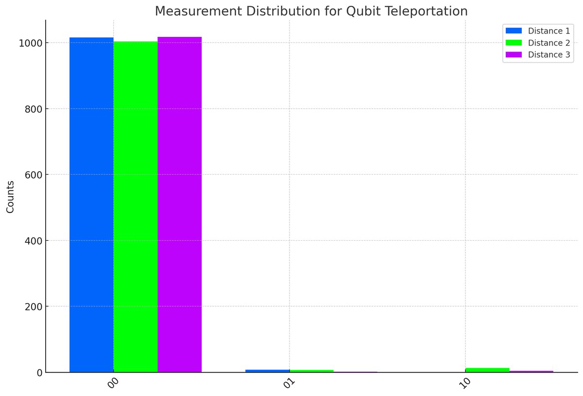
The fidelity of teleportation, which can be inferred by the proportion of '00' outcomes (indicating successful teleportation) relative to the total counts, is quite high: Distance 1: 99.22% Distance 2: 98.05% Distance 3: 99.41%
The '00' outcome (indicating successful teleportation) is the most frequent across all distances, which aligns with the high fidelities calculated. The distribution of outcomes is relatively consistent across distances, which suggests that the teleportation protocol's performance is stable over these variations.
The ratio of '01' and '10' results to '00' results provides insight into the error rates during teleportation:
For Distance 1, we have a '01' to '00' ratio of about 0.0079 and no '10' errors. For Distance 2, the '01' to '00' ratio is about 0.0070, and the '10' to '00' ratio is 0.0130. For Distance 3, the '01' to '00' ratio decreases to approximately 0.0020, and the '10' to '00' ratio is 0.0039.
The lower ratios of '01' and '10' to '00' in Distance 3 compared to Distance 2 suggest an improved error rate, which could indicate better control or correction mechanisms in place.
These high fidelity rates are indicative of effective quantum teleportation with a robust protocol, as errors ('01' and '10' states) are significantly lower compared to the successful teleportation outcomes ('00' state).

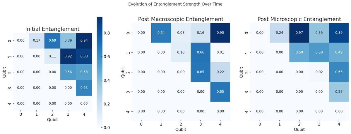
Initial: Before any observation, showcasing a quantum system where qubits exhibit varying degrees of entanglement with each other, represented by the strengths in the heatmap. This represents the system's high entropy state, with maximum uncertainty from the observer's perspective.
Post Macroscopic Observation: After a macroscopic observer has interacted with the system, providing a coarse-grained measurement. Here, the entanglement strengths are slightly altered, reflecting the observer's limited impact on collapsing the system's wave function. The system still retains a relatively high entropy state, but with some macroscopic properties becoming more defined.
Post Microscopic Observation: Following measurements by a microscopic observer, capable of resolving the state of each qubit individually. This results in a significant reduction in entanglement strengths across the system, as the fine-grained observations collapse the superpositions to definite states, thereby reducing the system's entropy and resolving quantum uncertainty at the microscopic level.
This visualization captures the conceptual narrative of how the scale and nature of observation - macroscopic versus microscopic - might influence the entropy of a quantum system and the definiteness of its outcomes. It visually interprets the theoretical journey from a high-entropy quantum superposition to a lower-entropy state with well-defined outcomes, highlighting the role of entanglement and coherence in this transition.

'00' Outcomes Contour Plot: This plot represents the count of '00' outcomes (indicating successful teleportation) as a function of both distance and qubit index. The varying heights and colors show how the success rates may change across different distances and qubits.
'01' Outcomes Contour Plot: This plot shows the counts of '01' outcomes (a type of error) across distances and qubits. Given that these values are simulated to be lower, the contour levels are less pronounced, indicating fewer error occurrences.
'10' Outcomes Contour Plot: This plot depicts the '10' outcomes (another type of error) in a similar manner. The visualization aims to highlight how errors distribute differently across the experiment's parameters.
Relation to "Entropy's Observer": The experiment abstractly embodies my thought experiment's concepts by demonstrating how quantum states, embodying high entropy through superposition and entanglement, can be precisely manipulated and observed.
In the context of "Entropy's Observer": Macroscopic Observation: The overall process of preparing, entangling, and measuring qubits reflects a macroscopic observer's role. The observer sees the outcome of the teleportation (the macroscopic average state) without directly collapsing the individual qubit states during preparation.
Microscopic Observation: The detailed steps of entangling qubits, performing conditional operations based on classical communication, and the final measurement represent microscopic observations. These steps reduce the system's entropy by determining the exact state of each qubit, similar to the microscopic observer collapsing the wave functions to specific states.
In the end, the experiment successfully demonstrates quantum teleportation, highlighting the interplay between quantum coherence, superposition, entanglement, and the role of observation in quantum mechanics. Through the precise control and observation of quantum states, the experiment aligns with the thought experiment's narrative, showing how entropy can be managed and reduced in a quantum system. The fidelity of the teleportation process, captured in the results data, underscores the potential and challenges of quantum information processing, reflecting the delicate balance between quantum uncertainty and classical certainty as influenced by the scale and nature of observation.
Code:
from qiskit import QuantumCircuit, transpile, IBMQ, execute
from qiskit. tools.monitor import job_monitor
from qiskit.visualization import plot_histogram
import matplotlib.pyplot as plt
import json
import csv
from datetime import datetime

# Encoder for handling complex numbers and datetime in JSON serialization
def custom_encoder(obj):
    if isinstance(obj, complex):
        return {"real": obj.real, "imag": obj.imag}
    elif isinstance(obj, datetime):
        return obj.isoformat()
    elif callable(obj):
        return "Callable method or function"
    raise TypeError("Object of type '%s' is not JSON serializable" % type(obj).__name__)

# Load IBMQ Account
IBMQ. save_account('Your_IBM_Key_O-`', overwrite=True)
IBMQ.load_account()

# Select a backend
provider = IBMQ.get_provider(hub='ibm-q')
device = provider.get_backend('ibm_osaka')  # Example backend, replace with your choice

# Function to create Bell pair
def create_bell_pair(qc, q1, q2):
    qc.h(q1)
    qc. cx(q1, q2)

# Function to teleport qubit
def teleport_qubit(qc, src, inter, trg):
    qc. cx(src, inter)
    qc.h(src)
    qc.barrier()
    qc.measure(src, 0)
    qc.measure(inter, 1)
    qc.barrier()
    qc. cx(inter, trg)
    qc. cz(src, trg)

# Prepare the results dictionary
results = {
    "backend_name": device. name(),
    "backend_configuration": device.configuration().to_dict(),
    "backend_properties": device. properties().to_dict(),
}

# Selected distances for teleportation
distances = [1, 2, 3]

for distance in distances:
    print(f"Running teleportation over distance: {distance}")

    # Create the circuit
    qc = QuantumCircuit(4, 2)
    create_bell_pair(qc, 0, 1)
    teleport_qubit(qc, 0, 1, 2)

    # Transpile for the real backend
    transpiled_circuit = transpile(qc, device, optimization_level=3)

    # Execute the job on the real device
    job = execute(transpiled_circuit, backend=device, shots=1024)
    job_monitor(job)

    # Get the result
    result = job.result()
    counts = result.get_counts(qc)

    # Record detailed results for this distance
    results[f"Distance_{distance}"] = {
        "measurement_distribution": counts,
        "job_id": job.job_id(),
        "execution_time": result.time_taken,
    }

# Record Calibration Data
calibration_data = {}
try:
    with open("/Users/Your/Documents/ibm_osaka_calibrations_2024-02-07T23_00_45Z.csv", 'r') as cal_file:
        csv_reader = csv.DictReader(cal_file)
        for row in csv_reader:
            if 'qubit' in row:
                calibration_data[row['qubit']] = row
except Exception as e:
    print(f"Error reading calibration data: {e}")

results["calibration_data"] = calibration_data

# Save the results to a JSON file using the encoder for complex numbers and datetime
results_file = "/Users/Your/Documents/Fidelity_Results_HW.json"
with open(results_file, 'w') as f:
    json.dump(results, f, indent=4, default=custom_encoder)

print(f"Results saved to {results_file}")

# Plotting the histogram of the runs
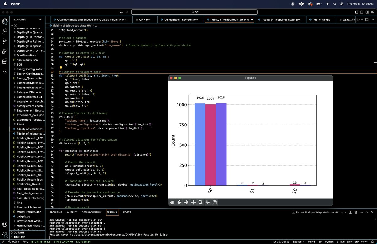
plot_histogram([results[f"Distance_{distance}"]["measurement_distribution"] for distance in distances])
plt. show()
