100-Qubit Quantum Entanglement on IBM's 127-Qubit Quantum Computer Osaka

This experiment, using qiskit and IBM's 127-Qubit Osaka, creates a quantum circuit to generate a complex entangled state across 100 qubits. It involves initializing the qubits, applying Hadamard and CNOT gates to create entanglement, and then performing ancilla-assisted and system wide measurements. The aim is to observe the behavior of this large-scale quantum system when subjected to specific quantum operations and measurements.

Code Walkthrough
1. Quantum Circuit Initialization:
The circuit is set up with 100 qubits. The first 5 qubits are designated as ancilla qubits, and the remaining 95 qubits are system qubits. Let ∣ψ_0⟩ represent the initial state of the entire circuit with 100 qubits.
Ancilla qubits:

∣ancilla⟩ = ∣00000⟩
This indicates that all 5 ancilla qubits are initialized in the quantum state |0⟩. System qubits:

∣system⟩ = ∣00000...⟩
This indicates that all 95 system qubits are initialized in the quantum state |0⟩.

2. Entanglement Generation:
The Hadamard gates H applied to each qubit create a superposition state. Mathematically, the action of a Hadamard gate on a single qubit is described by:

H∣0⟩ = 1/sqrt(2) * (∣0⟩ + ∣1⟩)

H∣1⟩ = 1/sqrt(2) * (∣0⟩ − ∣1⟩)
Applying the H gate to a qubit initially in the ∣0⟩ state, results in an equal superposition of ∣0⟩ and ∣1⟩.
The CNOT gates create entanglement between qubits. A CNOT gate is represented by the matrix:

CNOT = (1, 0, 0, 0, 0, 1, 0, 0, 0, 0, 0, 1, 0, 0, 1, 0)
The CNOT gate operates on two qubits: a control qubit and a target qubit. If the control qubit is in state ∣1⟩, the CNOT gate flips the target qubit's state, i.e., ∣0⟩ becomes ∣1⟩ and vice versa. If the control qubit is in state ∣0⟩, the target qubit remains unchanged.
When a CNOT gate is applied to a pair of qubits where the first (control) qubit is in a superposition (created by the H gate), it entangles the states of the two qubits. For example, if the control qubit is in the state (∣0⟩ + ∣1⟩)/sqrt(2) (after the H gate) and the target qubit is in state ∣0⟩, the CNOT operation will result in the entangled state (∣00⟩ + ∣11⟩)/sqrt(2)

3. Ancilla-Assisted Measurement:
We add additional ancilla qubits to indirectly measure the state of the system qubits. Additional CNOT gates entangle each ancilla qubit with a corresponding system qubit. The state of the system qubit affects the state of its paired ancilla qubit due to this entanglement. The measurement of a quantum state is a projection operation. When the ancilla qubits are measured, their state collapses to either ∣0⟩ or ∣1⟩. The measurement operators are M_0 = ∣0⟩⟨0∣ and M_1 = ∣1⟩, which project the qubit onto the ∣0⟩ and ∣1⟩ states respectively. This method helps in preserving the entangled state of the system qubits, as direct measurement would collapse their quantum state.

4. Measurement:
All qubits (both ancilla and system) are measured, collapsing their quantum states into classical bits. The measurement collapses the superposition of each qubit into a definite state, which can be 0 or 1. This collapse is probabilistic and is described by the Born rule. The Born Rule is a fundamental principle in quantum mechanics that provides the probability of observing a particular outcome. According to this rule, the probability P of measuring a qubit in state ∣0⟩ is P(∣0⟩) = ∣α∣^2, and similarly, the probability of measuring it in state ∣1⟩ is P(∣1⟩) = ∣β∣^2. Important to note that ∣α∣^2 + ∣β∣^2 = 1, ensuring the total probability sums up to 1.

5. Execution on Osaka:
The transpilation step optimizes the quantum circuit for execution on Osaka's hardware. This optimization involves decomposing gates into elementary gates, rearranging gates for optimal execution, and handling hardware-specific constraints. The experiment is executed for 1000 shots.

6. Result Analysis:
Complex numbers and datetime objects are handled using a custom JSON serialization function. All results and backend data are saved to a Json for further analysis.

Results:
Median: 6.05 * 10^29 Mean: 6.18 * 10^29 Standard Deviation: 3.61 * 10^29 The median offers a central value around which the quantum state measurements are distributed, while the mean provides an average value. The standard deviation indicates the amount of variation or dispersion in the quantum state measurements.
Top ten ancilla states: State 01000: 10.61% State 00111: 10.34% State 00110: 10.34% State 10110: 10.08% State 00000: 10.08% State 01010: 10.08% State 01110: 10.08% State 11010: 9.81% State 00100: 9.55% State 01101: 9.02%
Top three System States: 11011110100100110111101001101000011011111101111101011011110100011111111010011011011110010010001 (Observed 1 time) 10110011010001001010001001111111101100001101111111100000101011110100110111000010010011101001000 (Observed 1 time) 01000100011111111110111110010100100100110010111111101010011101010111101010010100100111100011000 (Observed 1 time)
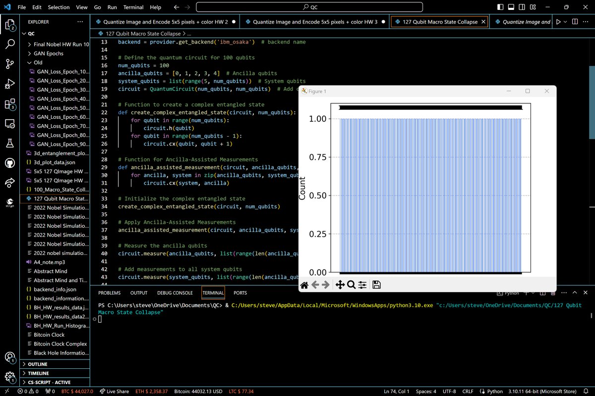
There were 1000 unique system states observed in the experiment. This high number of unique states suggests a rich diversity in the quantum states explored by the system qubits. Each of the top ten system states was observed only once. Given the total of 1000 unique states, this means the top states make up only 1% of all the unique states observed.
The diversity of the observed states in the system qubits indicates a high level of quantum coherence. In a coherent quantum system, qubits can exist in a superposition of many states, leading to a wide variety of possible outcomes upon measurement.
The broad distribution of system states suggests that the system qubits might be experiencing less pronounced decoherence compared to a scenario where a few states dominate (which would suggest a collapse into classical states).

Menger Sponge fractal: Above is a Menger Sponge fractal with an applied color gradient for normalized positions. The X, Y, and Z axes represent the fractal's dimensions, with the color gradient adding a visual cue to the depth and complexity of the structure. Each part of the fractal represents different states or stages in the quantum collapse process.
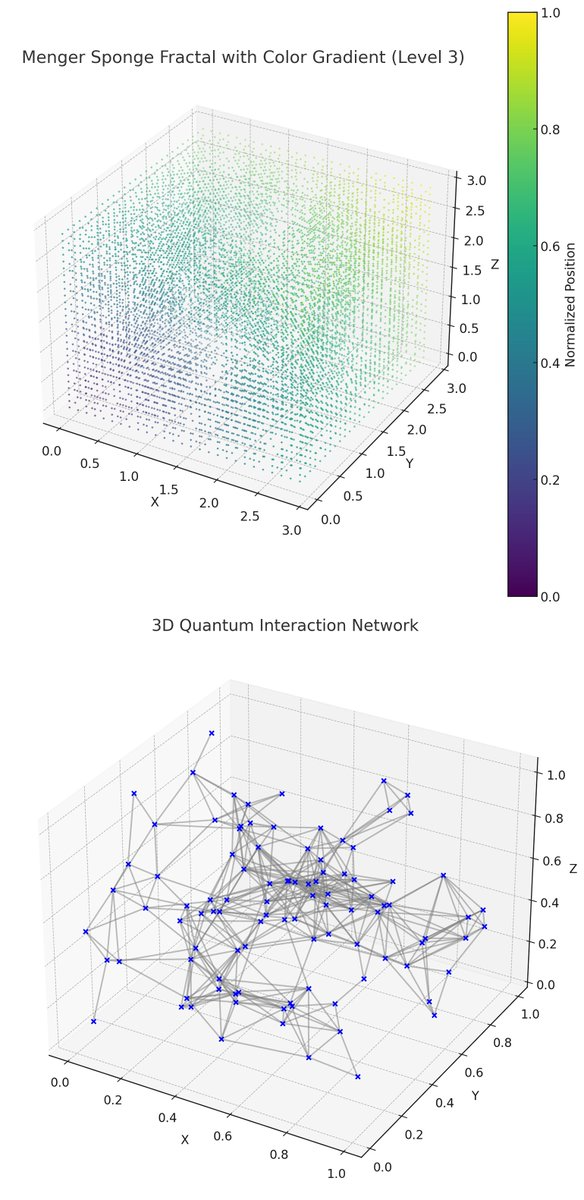
3D Quantum Interaction Network: Also above is a 3D Quantum Interaction Network using the results data. Each node (point in 3D space) represents a quantum state, with its position corresponding to state index and frequency. The links or edges between nodes symbolize transitions between states. The thickness and color of the links represent the strength and probability of these interactions.

Above is a 3D quantum harmonic oscillation visualization. Each oscillating element represents a quantum state, and its movement in 3D space illustrates the state's dynamic behavior over time. The amplitude and frequency of oscillation represents the quantum properties probability, amplitude, and energy levels. The color and size of each oscillating element can vary based on frequency of occurrence or a specific quantum metric.

Above is a 3D quantum tunneling representation rendered from our experiment data. Lines or paths connect different quantum states, representing transitions between these states. The curvature of the paths visualizes the transition process. The color intensity of each path, using the Viridis colormap, represents the probability or frequency of transitions. Darker colors indicate more frequent transitions.
In the end, a 100-qubit quantum circuit was designed and executed to capture the behavior of quantum entanglement on a large scale. We learned that the quantum circuit, initialized with both ancilla and system qubits in the |0⟩ state, demonstrates distinct behaviors between these two sets of qubits. The ancilla qubits, used here for indirect measurements, showed a higher frequency of certain states, indicating their stable and consistent role in the quantum circuit. In contrast, the system qubits exhibited a rich diversity of states, suggesting complex quantum dynamics and a higher degree of quantum coherence in this system.

Code:

# Imports
import json
from datetime import datetime
from qiskit import QuantumCircuit, execute, transpile, IBMQ
from qiskit.visualization import plot_histogram
from qiskit_ibm_provider import IBMProvider
import matplotlib.pyplot as plt

# Enter your IBMQ API key here
ibm_api_key = 'Your_API_Key_Mfer'
provider = IBMProvider(ibm_api_key)

# backend name
backend = provider.get_backend('ibm_osaka')  

# Define the quantum circuit for 100 qubits
num_qubits = 100
ancilla_qubits = [0, 1, 2, 3, 4]  # Ancilla qubits
system_qubits = list(range(5, num_qubits))  # System qubits
circuit = QuantumCircuit(num_qubits, num_qubits)  # Add classical bits for measurement

# Function to create a complex entangled state
def create_complex_entangled_state(circuit, num_qubits):
    for qubit in range(num_qubits):
        circuit.h(qubit)
    for qubit in range(num_qubits - 1):
        circuit. cx(qubit, qubit + 1)

# Function for Ancilla-Assisted Measurements
def ancilla_assisted_measurement(circuit, ancilla_qubits, system_qubits):
    for ancilla, system in zip(ancilla_qubits, system_qubits):
        circuit. cx(system, ancilla)

# Initialize the complex entangled state
create_complex_entangled_state(circuit, num_qubits)

# Apply Ancilla-Assisted Measurements
ancilla_assisted_measurement(circuit, ancilla_qubits, system_qubits)

# Measure the ancilla qubits
circuit.measure(ancilla_qubits, list(range(len(ancilla_qubits))))

# Add measurements to all system qubits
circuit.measure(system_qubits, list(range(len(ancilla_qubits), num_qubits)))

# Execute the circuit on the quantum computer
transpiled_circuit = transpile(circuit, backend)
job = execute(transpiled_circuit, backend, shots=1000)
result = job.result()

# Function to handle complex numbers and datetime objects for JSON serialization
def complex_to_json(obj):
    if isinstance(obj, complex):
        return {"real": obj.real, "imag": obj.imag}
    if isinstance(obj, datetime):
        return obj.isoformat()  # Convert datetime objects to ISO format
    raise TypeError(f"Object of type {obj.__class__.__name__} is not JSON serializable")

# Display histogram of the results
plot_histogram(result.get_counts(circuit))
plt. show()

# Prepare data for JSON serialization
data = {
    "raw_counts": result.get_counts(circuit),
    "backend_properties": backend. properties().to_dict()
}

# Specified path for saving the results
json_path = 'c:\\Users\\Desktop\\100_Macro_State_Collapse_results.json'

# Serialize and save the data to a JSON file
with open(json_path, "w") as f:
    json.dump(data, f, default=complex_to_json)

print(f"Results saved to {json_path}")