Encoding Visual Data in 25 Quantum States on IBM's 127-Qubit Quantum Computer Osaka
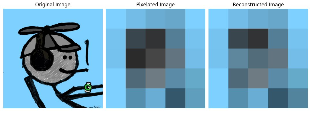
This experiment, using IBM's 127-qubit quantum computer Osaka and Qiskit, aims to process a classical image using quantum measurement. The experiment involves encoding the color information of each pixel's RGB content of a classical image into quantum states, performing quantum measurements, and reconstructing the image based on the outcomes of those measurements. If the majority of the outcomes are '1', assign the corresponding normalized RGB values back to the pixel. If '0's are in the majority or there's an equal number of '0's and '1's, set the pixel to black. To get back the full image, including '0's, we apply a classical interpolation technique. For each black pixel or '0' run result, we replace it with the average color of its non-black neighboring pixels or '1's. This type of post error correction and classical integration can make up for some of the uncertainty in quantum mechanics.
Code Walkthrough
1. Classical Image Preprocessing:
First, a classical digital image is loaded and resized to a 5x5 grid.
The original image be represented as I_(original), and the resized image as I_(resized).
2. Color Encoding into Quantum States:
For each pixel in I_(resized), extract the RGB values, R, G, B, each ranging from 0 to 255.
Normalize these values to the range [0, 1] by dividing by 255.
We create a quantum circuit with three qubits, each representing one color channel (Red, Green, Blue). Initialize the qubits in the state ∣000⟩.
Apply rotation gates to encode the color information into the quantum state.
The rotation gates used are Rx(θ_R), Ry(θ_G), Rz(θ_B), where the rotation angles θ are calculated as θ_(color) = 2π * normalized color value.
The final state of each qubit after these rotations is: ∣000⟩∣ψ⟩ = Rx(θ_R) * Ry(θ_G) * Rz(θ_B) * ∣000⟩
This state is a superposition of the basis states ∣000⟩, ∣001⟩, ∣010⟩, …, ∣111⟩, with complex amplitudes dependent on the rotation angles.
3. Quantum Measurement:
The quantum circuit is measured in the computational basis (∣0⟩ and ∣1⟩).
We perform multiple measurements (shots) to gather probabilistic outcomes. The probability of measuring a state ∣q_2 * q_1 * q_0⟩ is given by ∣⟨q_2 * q_1 * q_0 * ∣ψ⟩∣^2.
The color of each pixel in the reconstructed image is determined based on the majority of outcomes in these measurements.
4. Image Reconstruction and Post-Processing:
We construct a new image I_(reconstructed) based on the measurement results.
If the majority of the outcomes are '1', assign the corresponding normalized RGB values back to the pixel.
If '0's are in the majority or there's an equal number of '0's and '1's, set the pixel to black.
To get back the full image, including '0's, we apply a classical interpolation technique to enhance the reconstructed image. For each black pixel, replace it with the average color of its non-black neighboring pixels.
For each identified black pixel, the algorithm examines its immediate neighbors. In a 2D grid, each pixel (except those on the edges) has eight neighbors (top, bottom, left, right, and four diagonals).
We extract the color information (RGB values) of these neighboring pixels.
We then compute the average color of the non-black neighboring pixels. This is done to avoid the influence of other black pixels and to obtain a color representative of the surrounding area.
Mathematically, if C_1, C_2, …, C_n are the RGB values of the non-black neighboring pixels, the average color C_(avg) is calculated as: C_(avg) = (1/n) * ∑ i=1 n (C_i)
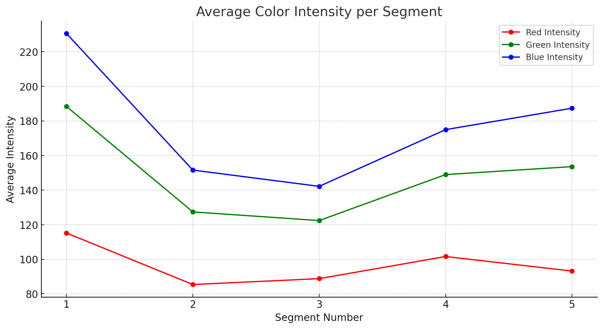
This calculation is performed separately for each color channel (Red, Green, and Blue) to obtain the average RGB value.
5. Result Analysis and Comparison:
Analyze I_(reconstructed) in comparison with I_(original) and I_(resized) to assess the effectiveness of quantum image processing.
We also save all result data, including the average colors and measurement results, to a json file for analysis.


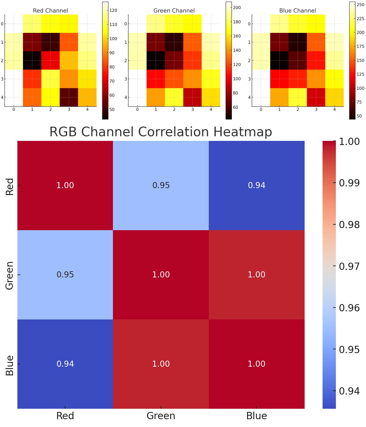
RGB Channel Correlation Heatmap (bottom): This heatmap displays the correlation coefficients between the red, green, and blue channels. The values range from -1 to 1, where 1 indicates a perfect positive correlation, -1 indicates a perfect negative correlation, and 0 means no correlation. This visualization helps in understanding how the different color channels are related to each other in terms of their intensities.

In the end, this experiment provides a novel look into how quantum computing can be harnessed for tasks like image processing, highlighting the probabilistic nature of quantum measurements and the need for integrating quantum and classical methods for practical applications.
Code:
# Importing necessary libraries
import cv2
import numpy as np
import matplotlib.pyplot as plt
from qiskit import QuantumCircuit, Aer, execute, IBMQ
from qiskit.visualization import plot_histogram
from qiskit.quantum_info import Statevector
from qiskit.providers.ibmq import least_busy
from qiskit. tools.monitor import job_monitor
from qiskit.ignis.mitigation.measurement import (complete_meas_cal, CompleteMeasFitter)
import json

# Function to encode RGB values into quantum statevectors
def encode_rgb_to_statevector(red, green, blue):
    normalized_red = red / 255.0
    normalized_green = green / 255.0
    normalized_blue = blue / 255.0

    qc = QuantumCircuit(3)
    qc.rx(2 * np.pi * normalized_red, 0)   # Encode red intensity
    qc.ry(2 * np.pi * normalized_green, 1) # Encode green intensity
    qc.rz(2 * np.pi * normalized_blue, 2)  # Encode blue intensity

    return Statevector.from_instruction(qc)

# Selecting a quantum provider and backend
IBMQ. save_account('Your_IBM_Accout_Mfer', overwrite=True)
IBMQ.load_account()
provider = IBMQ.get_provider(hub='ibm-q')
backend = provider.get_backend('ibm_osaka')
print("Using backend: ", backend)

# Loading and processing an image
image_path = "C:\\Users\\Pictures\\Blue mfer.jpg"
original_image = cv2.imread(image_path)
original_image_rgb = cv2.cvtColor(original_image, cv2.COLOR_BGR2RGB)

# Setting parameters for image processing
grid_size = 5
block_size = 1

resized_image = cv2.resize(original_image_rgb, (grid_size, grid_size), interpolation=cv2.INTER_AREA)

# Initializing lists to store average colors and measurement results
avg_colors = []
measurement_results = []

# Setting up calibration circuits for measurement error mitigation
cal_circuits, state_labels = complete_meas_cal(qr=QuantumCircuit(3).qregs[0], circlabel='measerrormitigationcal')
cal_jobs = execute(cal_circuits, backend=backend, shots=5)
job_monitor(cal_jobs)
cal_results = cal_jobs.result()
meas_fitter = CompleteMeasFitter(cal_results, state_labels)

# Processing each pixel of the resized image
for i in range(grid_size):
    for j in range(grid_size):
        color = resized_image[i, j]
        avg_colors.append(color)  # Storing the color of each pixel
        statevector = encode_rgb_to_statevector(color[0], color[1], color[2])
        qc = QuantumCircuit(3)
        qc.initialize(statevector. data, [0, 1, 2])
        qc.measure_all()
        job = execute(qc, backend=backend, shots=5)
        job_monitor(job)
        result = job.result()
        counts = result.get_counts(qc)
        measurement_results.append(1 if '1' in max(counts, key=counts.get) else 0)

# Reconstructing the image based on measurement results
reconstructed_image = np.zeros((grid_size * block_size, grid_size * block_size, 3), dtype=np.uint8)
for i in range(grid_size):
    for j in range(grid_size):
        idx = i * grid_size + j
        if measurement_results[idx]:
            reconstructed_image[i*block_size:(i+1)*block_size, j*block_size:(j+1)*block_size] = np.array(avg_colors[idx], dtype=np.uint8)
        else:
            print(f"Grid Cell [{i},{j}] is set to black due to measurement result 0.")

# Function to interpolate black pixels in the image
def interpolate_black_pixels(image):
    height, width, _ = image.shape
    for i in range(height):
        for j in range(width):
            if np.all(image[i, j] == 0):  # If the pixel is black
                neighboring_colors = []
                for di in range(-1, 2):
                    for dj in range(-1, 2):
                        ni, nj = i + di, j + dj
                        if 0 <= ni < height and 0 <= nj < width and not (di == 0 and dj == 0):
                            if not np.all(image[ni, nj] == 0):
                                neighboring_colors.append(image[ni, nj])
                if neighboring_colors:
                    image[i, j] = np.mean(neighboring_colors, axis=0)
    return image

# Applying the interpolation function
interpolated_reconstructed_image = interpolate_black_pixels(reconstructed_image.copy())

# Plotting the original, pixelated, and reconstructed images
fig, axs = plt.subplots(1, 3, figsize=(15, 5))

axs[0].imshow(original_image_rgb)
axs[0].set_title('Original Image')
axs[0].axis('off')

axs[1].imshow(resized_image)
axs[1].set_title('Pixelated Image')
axs[1].axis('off')

axs[2].imshow(interpolated_reconstructed_image)
axs[2].set_title('Reconstructed Image')
axs[2].axis('off')

plt.tight_layout()
plt. show()

# Convert avg_colors to a list of lists (from a list of NumPy arrays)
avg_colors_list = [color.tolist() for color in avg_colors]

# Update the data to save
data_to_save = {
    'average_colors': avg_colors_list,
    'measurement_results': measurement_results
}

# Save the results to a JSON file
json_path = "C:\\Users\\Desktop\\127_5x5_quantum_image_processing_results.json"
with open(json_path, 'w') as json_file:
    json.dump(data_to_save, json_file, indent=4)
print(f"Results saved to {json_path}")
